
Setting up Quantiacs
- The Tech Platform

- Apr 6, 2021
- 2 min read
Quantiacs supports offline development of trading systems in Python 3 and Matlab which requires downloading the toolbox. Running your trading system and submitting it to win our competition has never been easier.
Python
Step 1: Download and install Python 3.7 on your machine. We recommend using Anaconda as it will reliably install all the necessary dependencies.
To download and install Anaconda, please follow the instructions on the installation page for Windows, MacOS and Linux.
Step 2 : Create a virtual environment for Quantiacs to install the toolbox and manage dependencies:
conda create --name quantiacsbox
conda activate quantiacsbox
conda install -c quantiacspkg quantiacstoolbox
Step 3: Launch Quantiacs by simply activating the Quantiacs environment using:
conda activate quantiacsboxLeave the environment using:
conda deactivateStep 4: Run a trading system.
We provide several public examples on github as a starting point. If you have downloaded the file trendFollowing.py in your directory, for example, then you can just go to that directory and type:
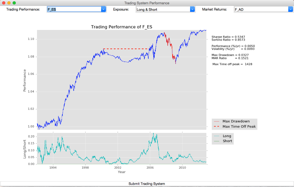
python trendFollowing.pyThis command will evaluate the sample system on the defined data set. After evaluation the toolbox will launch a dashboard with important performance indicators: the equity curve, the long vs short exposure, market-wise performance and the Sharpe Ratio:

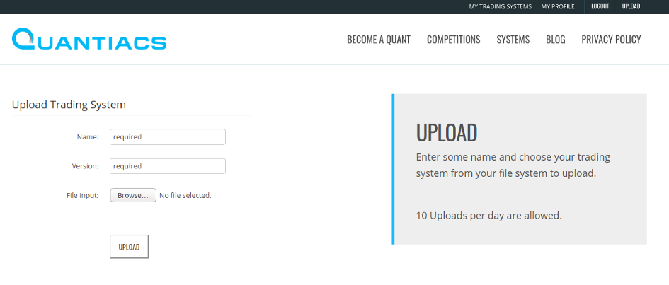
To take part in a Quantiacs competition (winners receive $2.25M USD in allocations), submit your strategy to our server. Simply login to your account, press the ‘Upload’ button to upload your file:

Your system will be backtested and its performance updated on a daily basis with fresh new data.
The Python toolbox supports several libraries:
numpy
pandas
keras
lightgbm
matplotlib
scikit-learn
scipy
seaborn
statsmodels
TA-lib
tensorflow
torch
xgboost
Matlab
To get the Matlab toolbox, download it from our page or from github. Add the opened zip-file to your Matlab search path. This will make the toolbox functions available from the command window.
With the toolbox in your Matlab search path, you can now backtest your trading algorithms. You can get started with sample algorithm examples on github. To evaluate the trend-following sample algorithm defined in the file trendfollowing.m you can simply type:
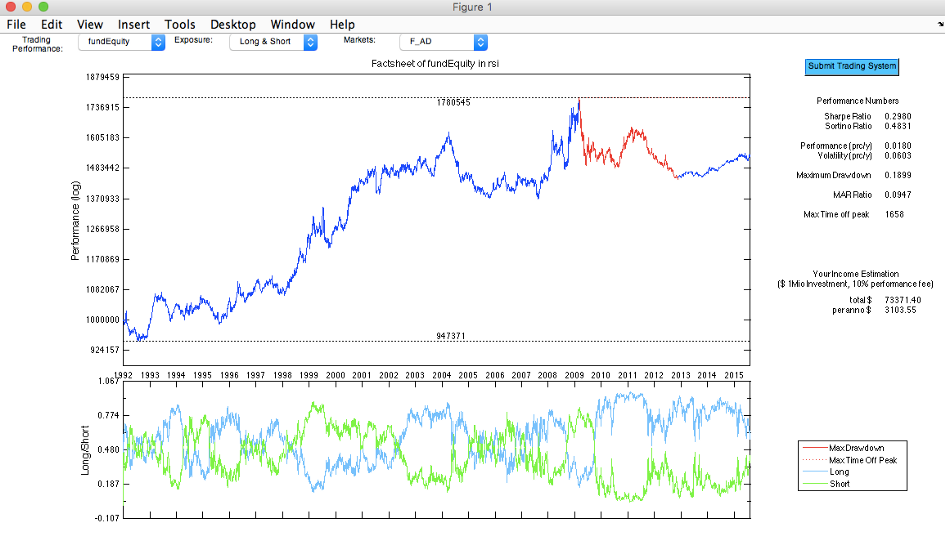
runts(‘trendfollowing.m’)This runs the evaluation of the sample system on the defined market list. Once the system is evaluated it opens a window with important performance indicators like the equity curve, the long vs short exposure, market-wise performance and the Sharpe Ratio:

Submitting the system can be made by logging in to your account, pressing the upload button and uploading your file as shown for Python files.
We support the following Matlab toolboxes:
Curve Fitting
Deep Learning
Econometrics
Financial
Global Optimization
Optimization
Signal Processing
Statistics and Machine Learning
Submitting systems before end of 2020 will allow you to take part to the live simulation period until end of April 2021. The top 3 performing algorithms, ranked according to Sharpe Ratio, will get allocations of $1M, $750k, and $500k USD.
Source: Medium
The Tech Platform


Comments