
Twitter Project- Classification using Multinomial Naive Bayes Classifier
- The Tech Platform

- Oct 6, 2020
- 4 min read


Hello Readers. Wondering what this Twitter project is about? I got this project as part of my course at Codecademy. Data and the files came bundled in and my job was to create a classification algorithm using tweet data collected from three different locations New York, London and Paris. I used Naive Bayes Classifier to build an algorithm which can classify from where the tweet or sentence came out of the three above mentioned locations. The scope of this project is limited to these three cities but concepts have wider application.
What is Multinomial Naive Bayes Classifier?
Naive Bayes classifier is a classification algorithm which works on Bayes theorem. It assumes that all the features exist independent of each other. It is supervised machine learning algorithm and we need to provide both data and labels to train it. It’s simplicity gives it speed but also makes it a poorer classifier. Let’s dive in to our project then.
Loading and Investigating data
I used Jupyter notebook for this project and started with loading the data and studying features, data types, whether data needs cleaning, how many data entries are there, this will give us a general sense of data. Following code will do the job of importing pandas and loading data into variables.
import pandas as pdnew_york_tweets = pd.read_json(r'data\new_york.json', lines = True)
london_tweets = pd.read_json(r'data\london.json', lines = True)
paris_tweets = pd.read_json(r'data\paris.json', lines = True)
New York, Paris and London data sets had 4723, 5341 and 2510 data entries respectively for text which contains tweets by users. There were a total of 35 columns in each data set which I have not named to avoid boredom.
Classifying text and combining data
Before we can start making any sort of algorithm we will need to combine all the text we extracted, which is stored in a column named text, into one long list with labels 0,1 and 2 for New York, London and Paris tweets. Following code will get the job done.
new_york_text = new_york_tweets["text"].tolist()
london_text = london_tweets['text'].tolist()
paris_text = paris_tweets['text'].tolist()
all_tweets = new_york_text + london_text + paris_text
labels = [0] * len(new_york_text) + [1] * len(london_text) + [2] * len(paris_text)
Making training and test set
Next step will be to prepare the data we have and split it into training and test sets. We will train our model using training data and training labels and then we will test it using test data and test labels. Scikit learn’s train_test_split function is perfect for this job.
from sklearn.model_selection import train_test_splittrain_data, test_data, train_labels, test_labels = train_test_split(all_tweets, labels, test_size = 0.2, random_state=1)Making Count Vectors
To use Naive Bayes Classifier we will have to change our text data into vectors where a sentence like “ Home sweet home baby” will be changed to a list where home will have 2 as it appears twice, sweet will be 1 and baby will be 1 as well and many 0’s will follow as these will represent the words which did not appear in the text but are part of training data set.
We will start by creating a model named counter using CountVectorizer(), then we will fit this model with training data to teach it our vocabulary and transform our data in the training and test data sets.
from sklearn.feature_extraction.text import CountVectorizercounter = CountVectorizer()
counter.fit(train_data)
train_counts = counter.transform(train_data)
test_counts = counter.transform(test_data)
Train and Test Multi NB Classifier
Now we will train our model using train_data and train_labels and then we will use the trained model to predict what should be labels for our test_data. Training the model will be done using .fit() and prediction on test data will be made using .predict().
from sklearn.naive_bayes import MultinomialNBclassifier = MultinomialNB()
classifier.fit(train_counts,train_labels)
predictions = classifier.predict(test_counts)
Evaluate the model
To know how accurate our model is in predicting the location of tweets we need to calculate its accuracy this we will achieve through accuracy_score which is part of sklearn.metrics.
from sklearn.metrics import accuracy_scoreaccuracy = accuracy_score(test_labels,predictions)The above code gives us an accuracy of 67.8%, cool isn’t it. We passed. If you are feeling dissatisfied with percentage accuracy then hold on for few lines we will dig into the reasons behind it. There is another test which we can use to know the accuracy of our model. It is called confusion matrix.
What is confusion matrix?
A confusion matrix is a matrix which causes confusion. Kiddin! It is a matrix which shows us which data points were predicted what. In our case we will get the data like this:
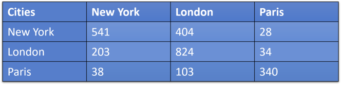
Confusion Matrix Source: Original
This can be interpreted as number of New York tweets that were classified as New York-541, London-404 and Paris-28. Number of London posts that were classified as New York-203, London-824, and Paris-34. Number of tweets that were from Paris but were classified as New York-38, London-103 and Paris-340. There seems to be little misunderstanding when it comes to deciding whether a tweet is from New York or London. Wondering why well one of the reasons can be that both are English speaking cities and that is why they are little harder to distinguish. That was also the reason why we had 67.8% accuracy.
Now that you have a basic understanding of what is going on continue exploring more ways of working with text data and classifications.
Source: medium.com


Comments