
QUERY OPTIMIZATION IN SQL
- The Tech Platform

- Oct 14, 2020
- 9 min read
Query optimization is a feature of many relational database management systems and other databases such as graph databases. The query optimizer attempts to determine the most efficient way to execute a given query by considering the possible query plans.
The query optimizer cannot be accessed directly by users: once queries are submitted to the database server, and parsed by the parser, they are then passed to the query optimizer where optimization occurs. However, some database engines allow guiding the query optimizer with hints.
Components of the Query Optimizer
The query optimizer operations include:
Query Transformation
Estimation
Plan Generation

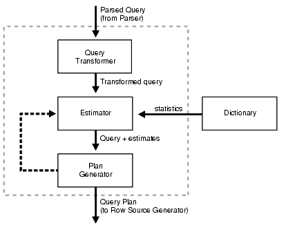
Query Optimization Components
Query Transformation
Each query portion of a statement is called a query block. The input to the query transformer is a parsed query, which is represented by a set of query blocks.
In the following example, the SQL statement consists of two query blocks. The subquery in parentheses is the inner query block. The outer query block, which is the rest of the SQL statement, retrieves names of employees in the departments whose IDs were supplied by the subquery.
SELECT first_name, last_name FROM employees WHERE department_id IN (SELECT department_id FROM departments WHERE location_id = 1800); The query form determines how query blocks are interrelated. The transformer determines whether it is advantageous to rewrite the original SQL statement into a semantically equivalent SQL statement that can be processed more efficiently.
The query transformer employs several query transformation techniques, including the following:
View Merging
Predicate Pushing
Subquery Unnesting
Query Rewrite with Materialized Views
Any combination of these transformations can apply to a given query.
1. View Merging Each view referenced in a query is expanded by the parser into a separate query block. The block essentially represents the view definition, and thus the result of a view. One option for the optimizer is to analyze the view query block separately and generate a view subplan. The optimizer then processes the rest of the query by using the view subplan to generate an overall query plan. This technique usually leads to a suboptimal query plan because the view is optimized separately.
In view merging, the transformer merges the query block representing the view into the containing query block. For example, suppose you create a view as follows:
CREATE VIEW employees_50_vw AS SELECT employee_id, last_name, job_id, salary, commission_pct, department_id FROM employees WHERE department_id = 50; You then query the view as follows:
SELECT employee_id FROM employees_50_vw WHERE employee_id > 150; The optimizer can use view merging to transform the query of employees_50_vw into the following equivalent query:
SELECT employee_id FROM employees WHERE department_id = 50 AND employee_id > 150; The view merging optimization applies to views that contain only selections, projections, and joins. That is, mergeable views do not contain set operators, aggregate functions, DISTINCT, GROUP BY, CONNECT BY, and so on.
To enable the optimizer to use view merging for any query issued by the user, you must grant the MERGE ANY VIEW privilege to the user. Grant the MERGE VIEW privilege to a user on specific views to enable the optimizer to use view merging for queries on these views. These privileges are required only under specific conditions, such as when a view is not merged because the security checks fail.
2. Predicate Pushing In predicate pushing, the optimizer "pushes" the relevant predicates from the containing query block into the view query block. For views that are not merged, this technique improves the subplan of the unmerged view because the database can use the pushed-in predicates to access indexes or to use as filters. For example, suppose you create a view that references two employee tables. The view is defined with a compound query that uses the UNION set operator, as follows:
CREATE VIEW all_employees_vw AS ( SELECT employee_id, last_name, job_id, commission_pct, department_id FROM employees ) UNION ( SELECT employee_id, last_name, job_id, commission_pct, department_id FROM contract_workers ); You then query the view as follows:
SELECT last_name FROM all_employees_vw WHERE department_id = 50; Because the view is a compound query, the optimizer cannot merge the view's query into the accessing query block. Instead, the optimizer can transform the accessing statement by pushing its predicate, the WHERE clause condition department_id=50, into the view's compound query. The equivalent transformed query is as follows:
SELECT last_name FROM ( SELECT employee_id, last_name, job_id, commission_pct, department_id FROM employees WHERE department_id=50 UNION SELECT employee_id, last_name, job_id, commission_pct, department_id FROM contract_workers WHERE department_id=50 ); 3. Subquery Unnesting In subquery unnesting, the optimizer transforms a nested query into an equivalent join statement, and then optimizes the join. This transformation enables the optimizer to take advantage of the join optimizer technique. The optimizer can perform this transformation only if the resulting join statement is guaranteed to return exactly the same rows as the original statement, and if subqueries do not contain aggregate functions such as AVG.
For example, suppose you connect as user sh and execute the following query:
SELECT * FROM sales WHERE cust_id IN ( SELECT cust_id FROM customers ); Because the customers.cust_id column is a primary key, the optimizer can transform the complex query into the following join statement that is guaranteed to return the same data:
SELECT sales.* FROM sales, customers WHERE sales.cust_id = customers.cust_id; If the optimizer cannot transform a complex statement into a join statement, it selects execution plans for the parent statement and the subquery as though they were separate statements. The optimizer then executes the subquery and uses the rows returned to execute the parent query. To improve execution speed of the overall query plan, the optimizer orders the subplans efficiently.
4. Query Rewrite with Materialized Views A materialized view is like a query with a result that the database materializes and stores in a table. When the database finds a user query compatible with the query associated with a materialized view, then the database can rewrite the query in terms of the materialized view. This technique improves query execution because most of the query result has been precomputed.
The query transformer looks for any materialized views that are compatible with the user query and selects one or more materialized views to rewrite the user query. The use of materialized views to rewrite a query is cost-based. That is, the optimizer does not rewrite the query if the plan generated without the materialized views has a lower cost than the plan generated with the materialized views.
Consider the following materialized view, cal_month_sales_mv, which aggregates the dollar amount sold each month:
CREATE MATERIALIZED VIEW cal_month_sales_mv ENABLE QUERY REWRITE AS SELECT t.calendar_month_desc, SUM(s.amount_sold) AS dollars FROM sales s, times t WHERE s.time_id = t.time_id GROUP BY t.calendar_month_desc; Assume that sales number is around one million in a typical month. The view has the precomputed aggregates for the dollar amount sold for each month. Consider the following query, which asks for the sum of the amount sold for each month:
SELECT t.calendar_month_desc, SUM(s.amount_sold) FROM sales s, times t WHERE s.time_id = t.time_id GROUP BY t.calendar_month_desc; Without query rewrite, the database must access sales directly and compute the sum of the amount sold. This method involves reading many million rows from sales, which invariably increases query response time. The join also further slows query response because the database must compute the join on several million rows. With query rewrite, the optimizer transparently rewrites the query as follows:
SELECT calendar_month, dollars FROM calendar_month_sales_mv; Estimation
The estimator determines the overall cost of a given execution plan. The estimator generates three different types of measures to achieve this goal:
Selectivity This measure represents a fraction of rows from a row set. The selectivity is tied to a query predicate, such as last_name='Smith', or a combination of predicates.
Cardinality This measure represents the number of rows in a row set.
Cost This measure represents units of work or resource used. The query optimizer uses disk I/O, CPU usage, and memory usage as units of work.
If statistics are available, then the estimator uses them to compute the measures. The statistics improve the degree of accuracy of the measures.
1. Selectivity The selectivity represents a fraction of rows from a row set. The row set can be a base table, a view, or the result of a join or a GROUP BY operator. The selectivity is tied to a query predicate, such as last_name = 'Smith', or a combination of predicates, such as last_name = 'Smith' AND job_type = 'Clerk'. A predicate filters a specific number of rows from a row set. Thus, the selectivity of a predicate indicates how many rows pass the predicate test. Selectivity ranges from 0.0 to 1.0. A selectivity of 0.0 means that no rows are selected from a row set, whereas a selectivity of 1.0 means that all rows are selected. A predicate becomes more selective as the value approaches 0.0 and less selective (or more un-selective) as the value approaches 1.0.
The optimizer estimates selectivity depending on whether statistics are available:
Statistics not available Depending on the value of the OPTIMIZER_DYNAMIC_SAMPLING initialization parameter, the optimizer either uses dynamic sampling or an internal default value. The database uses different internal defaults depending on the predicate type. For example, the internal default for an equality predicate (last_name = 'Smith') is lower than for a range predicate (last_name > 'Smith') because an equality predicate is expected to return a smaller fraction of rows.
Statistics available When statistics are available, the estimator uses them to estimate selectivity. Assume there are 150 distinct employee last names. For an equality predicate last_name > 'Smith', selectivity is the reciprocal of the number n of distinct values of last_name, which in this example is .006 because the query selects rows that contain 1 out of 150 distinct values. If a histogram is available on the last_name column, then the estimator uses the histogram instead of the number of distinct values. The histogram captures the distribution of different values in a column, so it yields better selectivity estimates, especially for columns that contain skewed data.
2. Cardinality Cardinality represents the number of rows in a row set. In this context, the row set can be a base table, a view, or the result of a join or GROUP BY operator.
3. Cost The cost represents units of work or resource used in an operation. The optimizer uses disk I/O, CPU usage, and memory usage as units of work. The operation can be scanning a table, accessing rows from a table by using an index, joining two tables together, or sorting a row set. The cost is the number of work units expected to be incurred when the database executes the query and produces its result. The access path determines the number of units of work required to get data from a base table. The access path can be a table scan, a fast full index scan, or an index scan.
Table scan or fast full index scan During a table scan or fast full index scan, the database reads multiple blocks from disk in a single I/O. Therefore, the cost of the scan depends on the number of blocks to be scanned and the multiblock read count value.
Index scan The cost of an index scan depends on the levels in the B-tree, the number of index leaf blocks to be scanned, and the number of rows to be fetched using the rowid in the index keys. The cost of fetching rows using rowids depends on the index clustering factor. See "Assessing I/O for Blocks, not Rows".
The join cost represents the combination of the individual access costs of the two row sets being joined, plus the cost of the join operation.
Plan Generation
The plan generator explores various plans for a query block by trying out different access paths, join methods, and join orders. Many plans are possible because of the various combinations of different access paths, join methods, and join orders that the database can use to produce the same result. The purpose of the generator is to pick the plan with the lowest cost.
1. Join Order A join order is the order in which different join items, such as tables, are accessed and joined together. Assume that the database joins table1, table2, and table3. The join order might be as follows:
The database accesses table1.
The database accesses table2 and joins its rows to table1.
The database accesses table3 and joins its data to the result of the join between table1 and table2.
2. Query Subplans The optimizer represents each nested subquery or unmerged view by a separate query block and generates a subplan. The database optimizes query blocks separately from the bottom up. Thus, the database optimizes the innermost query block first and generates a subplan for it, and then lastly generates the outer query block representing the entire query.
The number of possible plans for a query block is proportional to the number of join items in the FROM clause. This number rises exponentially with the number of join items. For example, the possible plans for a join of five tables will be significantly higher than the possible plans for a join of two tables.
3. Cutoff for Plan Selection The plan generator uses an internal cutoff to reduce the number of plans it tries when finding the lowest-cost plan. The cutoff is based on the cost of the current best plan. If the current best cost is large, then the plan generator explores alternative plans to find a lower cost plan. If the current best cost is small, then the generator ends the search swiftly because further cost improvement will not be significant.
The cutoff works well if the plan generator starts with an initial join order that produces a plan with cost close to optimal. Finding a good initial join order is a difficult problem.
Query Optimization Techniques in SQL: Tips and Tricks: https://www.thetechplatform.com/post/query-optimization-techniques-in-sql-server-tips-and-tricks
Resources: Oracle
The Tech Platform


Comments