PyCaret 2.1 is here — What’s new?
- The Tech Platform

- Aug 31, 2020
- 6 min read
We are excited to announce PyCaret 2.1 — update for the month of Aug 2020.
PyCaret is an open-source, low-code machine learning library in Python that automates the machine learning workflow. It is an end-to-end machine learning and model management tool that speeds up the machine learning experiment cycle and makes you 10x more productive.
In comparison with the other open-source machine learning libraries, PyCaret is an alternate low-code library that can be used to replace hundreds of lines of code with few words only. This makes experiments exponentially fast and efficient.
If you haven’t heard or used PyCaret before, please see our previous announcement to get started quickly.
Installing PyCaret
Installing PyCaret is very easy and takes only a few minutes. We strongly recommend using a virtual environment to avoid potential conflict with other libraries. See the following example code to create a conda environment and install pycaret within that conda environment:
# create a conda environment
conda create --name yourenvname python=3.6  # activate environment
conda activate yourenvname  # install pycaret
pip install pycaret # create notebook kernel linked with the conda environment
python -m ipykernel install --user --name yourenvname --display-name "display-name"
If you have PyCaret already installed, you can update it using pip:
pip install --upgrade pycaretPyCaret 2.1 Feature Summary
👉 Hyperparameter Tuning on GPU
In PyCaret 2.0 we have announced GPU-enabled training for certain algorithms (XGBoost, LightGBM and Catboost). What’s new in 2.1 is now you can also tune the hyper-parameters of those models on GPU.
# train xgboost using gpu
xgboost = create_model('xgboost', tree_method = 'gpu_hist')# tune xgboost
tuned_xgboost = tune_model(xgboost)
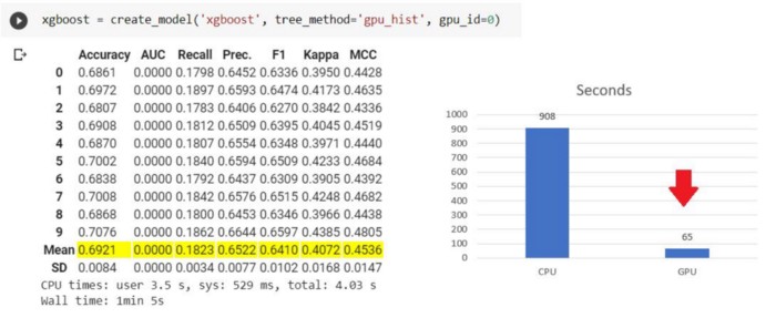
No additional parameter needed inside tune_model function as it automatically inherits the tree_method from xgboost instance created using the create_model function. If you are interested in little comparison, here it is:
100,000 rows with 88 features in a Multi-class problem with 8 classes
XGBoost Training on GPU (using Google Colab)
👉 Model Deployment
Since the first release of PyCaret in April 2020, you can deploy trained models on AWS simply by using the deploy_model from your Notebook. In the recent release, we have added functionalities to support deployment on GCP as well as Microsoft Azure.
Microsoft Azure
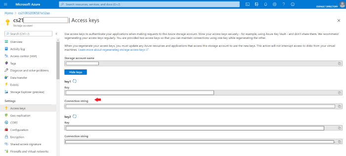
To deploy a model on Microsoft Azure, environment variables for connection string must be set. The connection string can be obtained from the ‘Access Keys’ of your storage account in Azure.
https:/portal.azure.com — Getting connection string from the storage account
Once you have copied the connection string, you can set it as an environment variable. See example below:
import os
os.environ['AZURE_STORAGE_CONNECTION_STRING'] = 'your-conn-string' from pycaret.classification import load_model
deploy_model(model = model, model_name = 'model-name', platform = 'azure', authentication = {'container' : 'container-name'})
BOOM! That’s it. Just by using one line of code, your entire machine learning pipeline is now shipped on the container in Microsoft Azure. You can access that using the load_model function.
import os
os.environ['AZURE_STORAGE_CONNECTION_STRING'] = 'your-conn-string' from pycaret.classification import load_model
loaded_model = load_model(model_name = 'model-name', platform = 'azure', authentication = {'container' : 'container-name'})from pycaret.classification import predict_model
predictions = predict_model(loaded_model, data = new-dataframe)
Google Cloud Platform
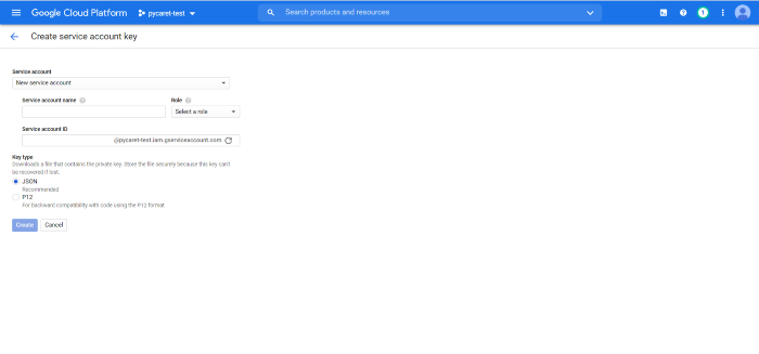
To deploy a model on Google Cloud Platform (GCP), you must create a project first either using a command line or GCP console. Once the project is created, you must create a service account and download the service account key as a JSON file, which is then used to set the environment variable.
Creating a new service account and downloading the JSON from GCP Console
To learn more about creating a service account, read the official documentation. Once you have created a service account and downloaded the JSON file from your GCP console you are ready for deployment.
import os
os.environ['GOOGLE_APPLICATION_CREDENTIALS'] = 'c:/path-to-json-file.json' from pycaret.classification import deploy_model
deploy_model(model = model, model_name = 'model-name', platform = 'gcp', authentication = {'project' : 'project-name', 'bucket' : 'bucket-name'})
Model uploaded. You can now access the model from the GCP bucket using the load_model function.
import os
os.environ['GOOGLE_APPLICATION_CREDENTIALS'] = 'c:/path-to-json-file.json' from pycaret.classification import load_model
loaded_model = load_model(model_name = 'model-name', platform = 'gcp', authentication = {'project' : 'project-name', 'bucket' : 'bucket-name'})from pycaret.classification import predict_model
predictions = predict_model(loaded_model, data = new-dataframe)
👉 MLFlow Deployment
In addition to using PyCaret’s native deployment functionalities, you can now also use all the MLFlow deployment capabilities. To use those, you must log your experiment using the log_experiment parameter in the setup function.
# init setup
exp1 = setup(data, target = 'target-name', log_experiment = True, experiment_name = 'exp-name')# create xgboost model
xgboost = create_model('xgboost')..
..
..# rest of your script# start mlflow server on localhost:5000
!mlflow ui
Now open https://localhost:5000 on your favorite browser.
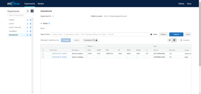
MLFlow UI on https://localhost:5000
You can see the details of run by clicking the “Start Time” shown on the left of “Run Name”. What you see inside is all the hyper-parameters and scoring metrics of a trained model and if you scroll down a little, all the artifacts are shown as well (see below).
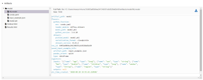
MLFLow Artifacts
A trained model along with other metadata files are stored under the directory “/model”. MLFlow follows a standard format for packaging machine learning models that can be used in a variety of downstream tools — for example, real-time serving through a REST API or batch inference on Apache Spark. If you want you can serve this model locally you can do that by using MLFlow command line.
mlflow models serve -m local-path-to-modelYou can then send the request to model using CURL to get the predictions.
curl http://127.0.0.1:5000/invocations -H 'Content-Type: application/json' -d '{
    "columns": ["age", "sex", "bmi", "children", "smoker", "region"],
    "data": [[19, "female", 27.9, 0, "yes", "southwest"]]
}'
(Note: This functionality of MLFlow is not supported on Windows OS yet).
MLFlow also provide integration with AWS Sagemaker and Azure Machine Learning Service. You can train models locally in a Docker container with SagMaker compatible environment or remotely on SageMaker.
To deploy remotely to SageMaker you need to set up your environment and AWS user account.
Example workflow using the MLflow CLI
mlflow sagemaker build-and-push-container
mlflow sagemaker run-local -m <path-to-model>
mlflow sagemaker deploy <parameters>
To learn more about all deployment capabilities of MLFlow, click here.
👉 MLFlow Model Registry
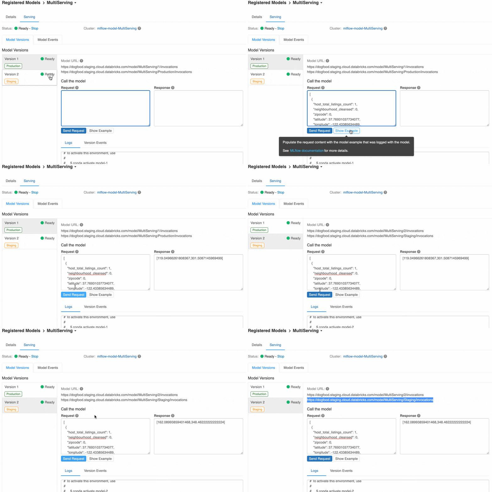
The MLflow Model Registry component is a centralized model store, set of APIs, and UI, to collaboratively manage the full lifecycle of an MLflow Model. It provides model lineage (which MLflow experiment and run produced the model), model versioning, stage transitions (for example from staging to production), and annotations.
If running your own MLflow server, you must use a database-backed backend store in order to access the model registry. Click here for more information. However, if you are using Databricks or any of the managed Databricks services such as Azure Databricks, you don’t need to worry about setting up anything. It comes with all the bells and whistles you would ever need.
👉 High-Resolution Plotting
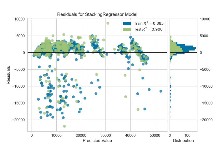
This is not ground-breaking but indeed a very useful addition for people using PyCaret for research and publications. The plot_model now has an additional parameter called “scale” through which you can control the resolution and generate high quality plot for your publications.
# create linear regression model
lr = create_model('lr')# plot in high-quality resolution
plot_model(lr, scale = 5) # default is 1
High-Resolution Residual Plot from PyCaret
👉 User-Defined Loss Function
This is one of the most requested feature ever since release of the first version. Allowing to tune hyper-parameters of a model using custom / user-defined function gives immense flexibility to data scientists. It is now possible to use user-defined custom loss functions using custom_scorer parameter in the tune_model function.
# define the loss function
def my_function(y_true, y_pred):
...
...# create scorer using sklearn
from sklearn.metrics import make_scorer
my_own_scorer = make_scorer(my_function, needs_proba=True)# train catboost model
catboost = create_model('catboost')# tune catboost using custom scorer
tuned_catboost = tune_model(catboost, custom_scorer = my_own_scorer)
👉 Feature Selection
Feature selection is a fundamental step in machine learning. You dispose of a bunch of features and you want to select only the relevant ones and to discard the others. The aim is simplifying the problem by removing unuseful features which would introduce unnecessary noise.
In PyCaret 2.1 we have introduced implementation of Boruta algorithm in Python (originally implemented in R). Boruta is a pretty smart algorithm dating back to 2010 designed to automatically perform feature selection on a dataset. To use this, you simply have to pass the feature_selection_method within the setup function.
exp1 = setup(data, target = 'target-var', feature_selection = True, feature_selection_method = 'boruta')To read more about Boruta algorithm, click here.
👉 Other Changes
blacklist and whitelist parameters in compare_models function is now renamed to exclude and include with no change in functionality.
To set the upper limit on training time in compare_models function, new parameter budget_time has been added.
PyCaret is now compatible with Pandas categorical datatype. Internally they are converted into object and are treated as the same way as object or bool is treated.
Numeric Imputation New method zero has been added in the numeric_imputation in the setup function. When method is set to zero, missing values are replaced with constant 0.
To make the output more human-readable, the Label column returned by predict_model function now returns the original value instead of encoded value.
To learn more about all the updates in PyCaret 2.1, please see the release notes.
There is no limit to what you can achieve using the lightweight workflow automation library in Python. If you find this useful, please do not forget to give us ⭐️ on our GitHub repo.
Source: Paper.li











Comments