
Machine Learning Workflow on Diabetes Data: Part 01
- The Tech Platform

- Feb 17, 2021
- 9 min read
“Machine learning in a medical setting can help enhance medical diagnosis dramatically.”


This article will portray how data related to diabetes can be leveraged to predict if a person has diabetes or not. More specifically, this article will focus on how machine learning can be utilized to predict diseases such as diabetes. By the end of this article series you will be able to understand concepts like data exploration, data cleansing, feature selection, model selection, model evaluation and apply them in a practical way.
What is Diabetes?
Diabetes is a disease that occurs when the blood glucose level becomes high, which ultimately leads to other health problems such as heart diseases, kidney disease, etc. Diabetes is caused mainly due to the consumption of highly processed food, bad consumption habits, etc. According to WHO, the number of people with diabetes has been increased over the years.
Prerequisites
Python 3.+
Anaconda (Scikit Learn, Numpy, Pandas, Matplotlib, Seaborn)
Jupyter Notebook.
Basic understanding of supervised machine learning methods: specifically classification.
Phase 0 — Data Preparation
As a Data Scientist, the most tedious task which we encounter is the acquiring and the preparation of a data set. Even though there is an abundance of data in this era, it is still hard to find a suitable data set that suits the problem you are trying to tackle. If there aren’t any suitable data sets to be found, you might have to create your own.
In this tutorial we aren’t going to create our own data set, instead, we will be using an existing data set called the “Pima Indians Diabetes Database” provided by the UCI Machine Learning Repository (famous repository for machine learning data sets). We will be performing the machine learning workflow with the Diabetes Data set provided above.
Phase 1 — Data Exploration
When encountered with a data set, first we should analyze and “get to know” the data set. This step is necessary to familiarize with the data, to gain some understanding of the potential features and to see if data cleaning is needed.
First, we will import the necessary libraries and import our data set to the Jupyter notebook. We can observe the mentioned columns in the data set.
%matplotlib inline
import pandas as pd
import numpy as np
import matplotlib.pyplot as plt
import seaborn as snsdiabetes = pd.read_csv('datasets/diabetes.csv')
diabetes.columns
Index(['Pregnancies', 'Glucose', 'BloodPressure', 'SkinThickness', 'Insulin', 'BMI', 'DiabetesPedigreeFunction', 'Age', 'Outcome'], dtype='object')
Important: It should be noted that the above data set contains only limited features, where as in reality numerous features come into play.
We can examine the data set using the pandas’ head() method.
diabetes.head()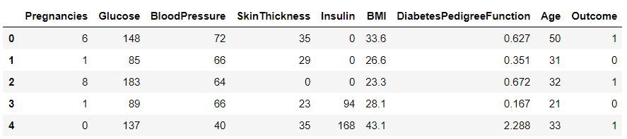
Fig — Diabetes data set
We can find the dimensions of the data set using the panda Dataframes’ ‘shape’ attribute.
print("Diabetes data set dimensions : {}".format(diabetes.shape))Diabetes data set dimensions : (768, 9)
We can observe that the data set contain 768 rows and 9 columns. ‘Outcome’ is the column which we are going to predict, which says if the patient is diabetic or not. 1 means the person is diabetic and 0 means a person is not. We can identify that out of the 768 persons, 500 are labeled as 0 (non-diabetic) and 268 as 1 (diabetic)
diabetes.groupby('Outcome').size()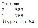
Fig— Class distribution
Visualization of data is an imperative aspect of data science. It helps to understand data and also to explain the data to another person. Python has several interesting visualization libraries such as Matplotlib, Seaborn, etc.
In this tutorial we will use pandas’ visualization which is built on top of matplotlib, to find the data distribution of the features.

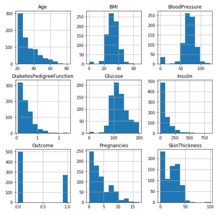
Fig— Data distribution
We can use the following code to draw histograms for the two responses separately. (The images are not displayed here.)
diabetes.groupby(‘Outcome’).hist(figsize=(9, 9))Phase 2— Data Cleaning
The next phase of the machine learning work flow is data cleaning. Considered to be one of the crucial steps of the workflow, because it can make or break the model. There is a saying in machine learning “Better data beats fancier algorithms”, which suggests better data gives you better resulting models.
There are several factors to consider in the data cleaning process.
Duplicate or irrelevant observations.
Bad labeling of data, same category occurring multiple times.
Missing or null data points.
Unexpected outliers.
We won’t be discussing about the data cleaning procedure in detail in this tutorial.
Since we are using a standard data set, we can safely assume that factors 1, 2 are already dealt with. Unexpected outliers are either useful or potentially harmful.
Missing or Null Data points
We can find any missing or null data points of the data set (if there is any) using the following pandas function.
diabetes.isnull().sum()
diabetes.isna().sum()
We can observe that there are no data points missing in the data set. If there were any, we should deal with them accordingly.
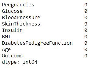
Fig — Observe missing data
Unexpected Outliers
When analyzing the histogram we can identify that there are some outliers in some columns. We will further analyze those outliers and determine what we can do about them.
Blood pressure: By observing the data we can see that there are 0 values for blood pressure. And it is evident that the readings of the data set seem wrong because a living person cannot have a diastolic blood pressure of zero. By observing the data we can see 35 counts where the value is 0.
print("Total : ", diabetes[diabetes.BloodPressure == 0].shape[0])Total :  35print(diabetes[diabetes.BloodPressure == 0].groupby('Outcome')['Age'].count())Outcome
0    19
1    16
Name: Age, dtype: int64
Plasma glucose levels: Even after fasting glucose levels would not be as low as zero. Therefore zero is an invalid reading. By observing the data we can see 5 counts where the value is 0.
print("Total : ", diabetes[diabetes.Glucose == 0].shape[0])Total :  5print(diabetes[diabetes.Glucose == 0].groupby('Outcome')['Age'].count())Total :  5
Outcome
0    3
1    2
Name: Age, dtype: int64
Skin Fold Thickness: For normal people, skin fold thickness can’t be less than 10 mm better yet zero. Total count where value is 0: 227.
print("Total : ", diabetes[diabetes.SkinThickness == 0].shape[0])Total :  227print(diabetes[diabetes.SkinThickness == 0].groupby('Outcome')['Age'].count())Outcome
0    139
1     88
Name: Age, dtype: int64BMI: Should not be 0 or close to zero unless the person is really underweight which could be life-threatening.
print("Total : ", diabetes[diabetes.BMI == 0].shape[0])Total :  11print(diabetes[diabetes.BMI == 0].groupby('Outcome')['Age'].count())Outcome
0    9
1    2
Name: Age, dtype: int64
Insulin: In a rare situation a person can have zero insulin but by observing the data, we can find that there is a total of 374 counts.
print("Total : ", diabetes[diabetes.Insulin == 0].shape[0])Total :  374print(diabetes[diabetes.Insulin == 0].groupby('Outcome')['Age'].count())Outcome
0    236
1    138
Name: Age, dtype: int64
Here are several ways to handle invalid data values :
Ignore/remove these cases: This is not actually possible in most cases because that would mean losing valuable information. And in this case “skin thickness” and “insulin” columns mean to have a lot of invalid points. But it might work for “BMI”, “glucose ”and “blood pressure” data points.
Put average/mean values: This might work for some data sets, but in our case putting a mean value to the blood pressure column would send a wrong signal to the model.
Avoid using features: It is possible to not use the features with a lot of invalid values for the model. This may work for “skin thickness” but it's hard to predict that.
By the end of the data cleaning process, we have come to the conclusion that this given data set is incomplete. Since this is a demonstration for machine learning we will proceed with the given data with some minor adjustments.
We will remove the rows which the “BloodPressure”, “BMI” and “Glucose” are zero.
diabetes_mod = diabetes[(diabetes.BloodPressure != 0) & (diabetes.BMI != 0) & (diabetes.Glucose != 0)]print(diabetes_mod.shape)(724, 9)Phase 3— Feature Engineering
Feature engineering is the process of transforming the gathered data into features that better represent the problem that we are trying to solve to the model, to improve its performance and accuracy.
Feature engineering creates more input features from the existing features and also combines several features to produce more intuitive features to feed to the model.
“ Feature engineering enables us to highlight the important features and facilitate to bring domain expertise on the problem to the table. It also allows avoiding overfitting the model despite providing many input features”.
The domain of the problem we are trying to tackle requires lots of related features. Since the data set is already provided, and by examining the data we can’t further create or dismiss any data at this point. In the data set, we have the following features.
‘Pregnancies’, ‘Glucose’, ‘Blood Pressure’, ‘Skin Thickness’, ‘Insulin’, ‘BMI’, ‘Diabetes Pedigree Function’, ‘Age’
By a crude observation, we can say that the ‘Skin Thickness’ is not an indicator of diabetes. But we can’t deny the fact that it is unusable at this point.
Therefore we will use all the features available. We separate the data set into features and the response that we are going to predict. We will assign the features to the X variable and the response to the y variable.
feature_names = ['Pregnancies', 'Glucose', 'BloodPressure', 'SkinThickness', 'Insulin', 'BMI', 'DiabetesPedigreeFunction', 'Age']X = diabetes_mod[feature_names]
y = diabetes_mod.Outcome
Generally feature engineering is performed before selecting the model. However, for this tutorial we follow a different approach. Initially, we will be utilizing all the features provided in the data set to the model, we will revisit features engineering to discuss feature importance on the selected model.
The given article gives a very good explanation of Feature Engineering.
Phase 4— Model Selection
Model selection or algorithm selection phase is the most exciting and the heart of machine learning. It is the phase where we select the model which performs best for the data set at hand.
First, we will be calculating the “Classification Accuracy (Testing Accuracy)” of a given set of classification models with their default parameters to determine which model performs better with the diabetes data set.
We will import the necessary libraries for the notebook. We import 7 classifiers namely K-Nearest Neighbors, Support Vector Classifier, Logistic Regression, Gaussian Naive Bayes, Random Forest, and Gradient Boost to be contenders for the best classifier.
from sklearn.neighbors import KNeighborsClassifier
from sklearn.svm import SVC
from sklearn.linear_model import LogisticRegression
from sklearn.tree import DecisionTreeClassifier
from sklearn.naive_bayes import GaussianNB
from sklearn.ensemble import RandomForestClassifier
from sklearn.ensemble import GradientBoostingClassifier
We will initialize the classifier models with their default parameters and add them to a model list.
models = []models.append(('KNN', KNeighborsClassifier()))
models.append(('SVC', SVC()))
models.append(('LR', LogisticRegression()))
models.append(('DT', DecisionTreeClassifier()))
models.append(('GNB', GaussianNB()))
models.append(('RF', RandomForestClassifier()))
models.append(('GB', GradientBoostingClassifier()))
Ex: Generally training the model with Scikit learn is as follows. knn = KNeighborsClassifier() knn.fit(X_train, y_train)
Evaluation Methods
It is a general practice to avoid training and testing on the same data. The reasons are that the goal of the model is to predict out-of-sample data, and the model could be overly complex leading to overfitting. To avoid the aforementioned problems, there are two precautions.
Train/Test Split
K-Fold Cross-Validation
We will import “train_test_split” for train/test split and “cross_val_score” for k-fold cross-validation. “accuracy_score” is to evaluate the accuracy of the model in the train/test split method.
from sklearn.model_selection import train_test_split
from sklearn.model_selection import cross_val_score
from sklearn.metrics import accuracy_score
We will perform the mentioned methods to find the best performing base models.
Train/Test Split
This method split the data set into two portions: a training set and a testing set. The training set is used to train the model. And the testing set is used to test the model, and evaluate the accuracy.
Pros : But, train/test split is still useful because of its flexibility and speed Cons : Provides a high-variance estimate of out-of-sample accuracy
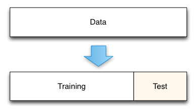
Fig — Train/Test Split
Train/Test Split with Scikit Learn :
Next, we can split the features and responses into train and test portions. We stratify (a process where each response class should be represented with equal proportions in each of the portions) the samples.
X_train, X_test, y_train, y_test = train_test_split(X, y, stratify = diabetes_mod.Outcome, random_state=0)Then we fit each model in a loop and calculate the accuracy of the respective model using the “accuracy_score”.
names = []
scores = []for name, model in models:
    model.fit(X_train, y_train)
    y_pred = model.predict(X_test)
    scores.append(accuracy_score(y_test, y_pred))
    names.append(name)tr_split = pd.DataFrame({'Name': names, 'Score': scores})
print(tr_split)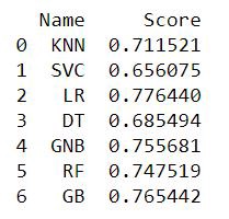
Fig — Train/Test Split Accuracy Scores
K-Fold Cross-Validation
This method splits the data set into K equal partitions (“folds”), then use 1 fold as the testing set and the union of the other folds as the training set. Then the model is tested for accuracy. The process will follow the above steps K times, using different folds as the testing set each time. The average testing accuracy of the process is the testing accuracy.
Pros : More accurate estimate of out-of-sample accuracy. More “efficient” use of data (every observation is used for both training and testing) Cons : Much slower than Train/Test split.

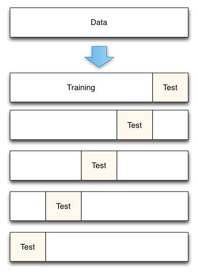
Fig— 5-Fold cross validation process
It is preferred to use this method where computation capability is not scarce. We will be using this method from here on out.
K-Fold Cross Validation with Scikit Learn :
We will move forward with K-Fold cross validation as it is more accurate and use the data efficiently. We will train the models using 10 fold cross validation and calculate the mean accuracy of the models. “cross_val_score” provides its own training and accuracy calculation interface.
names = []
scores = []for name, model in models:

    kfold = KFold(n_splits=10, random_state=10)
    score = cross_val_score(model, X, y, cv=kfold, scoring='accuracy').mean()

    names.append(name)
    scores.append(score)kf_cross_val = pd.DataFrame({'Name': names, 'Score': scores})
print(kf_cross_val)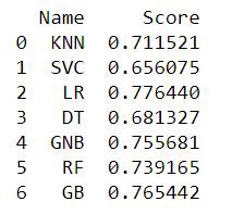
Fig — K-Fold Cross Validation Accuracy Scores
We can plot the accuracy scores using seaborn
axis = sns.barplot(x = 'Name', y = 'Score', data = kf_cross_val)
axis.set(xlabel='Classifier', ylabel='Accuracy')for p in axis.patches:
    height = p.get_height()
    axis.text(p.get_x() + p.get_width()/2, height + 0.005, '{:1.4f}'.format(height), ha="center")

plt.show()
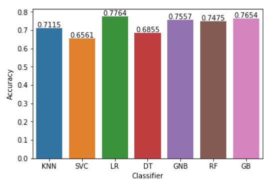
Fig — Accuracy of Classifiers
We can see the Logistic Regression, Gaussian Naive Bayes, Random Forest and Gradient Boosting have performed better than the rest. From the base level we can observe that the Logistic Regression performs better than the other algorithms.
At the baseline Logistic Regression managed to achieve a classification accuracy of 77.64 %. This will be selected as the prime candidate for the next phases.
Summary
In this article we discussed about the basic machine learning workflow steps such as data exploration, data cleaning steps, feature engineering basics and model selection using Scikit Learn library. In the next article I will be discussing more about feature engineering, and hyper parameter tuning.
Source: Medium
The Tech platform


hi