
How do you present your Data Science solution?
- The Tech Platform

- Aug 31, 2020
- 6 min read
An example of how to prepare a report on Credit Risk Modelling via Machine Learning


Its weekend time to try something new in Machine learning and make this time worthwhile. It is important to document the machine learning approach and solution to share it with the stakeholders, as much as it is to design it in the first place.
In today’s post, we will create a report on the ML solution on “Credit Risk Modelling” (the domain favoritism is evident here).
Let’s give it a shot.
The first and foremost important step is to understand the business objective thoroughly. What will be the expectation from the ML solution?
Preliminary set of questions:
How much data is available, does it have any pattern, will it be enough in predicting the target variable? Is there any other variable that plays a significant role in making the decision in real-life, but is not part of available data set? Can it be sourced or is there a way to proxy that information? Is the data made available to ML algorithm similar to the production data on which predictions will be generated? In other words, does train and test data come from similar distribution to learn the dependencies well enough to predict the unseen instances? And many more…
We will try to cover all these questions as we approach the problem, so tag along:
Objective:
To learn the association between the traits and attributes of different borrowers in history and their repayment status i.e. whether it resulted in Good Risk or Bad Risk.
Definition of Credit Risk:
It is the risk of witnessing defaults on a debt that may arise from a borrower failing to make required payments.
Target Variable:
Good (class 1, creditworthy) vs Bad (class 0, not creditworthy) Risk.
Data Description:
1000 records with 10 variables

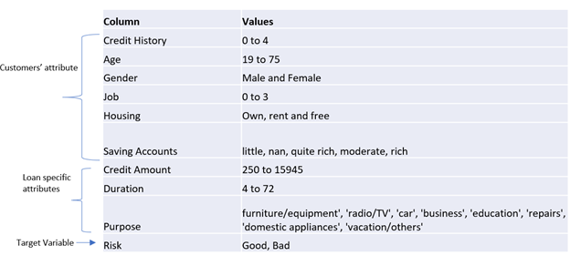
Data Description
Understanding the data is the key, make sure to understand the description of each variable, for example:
‘Credit History’ has 5 values (0 to 4), but how does its ordinality relates to the credit risk. Does a value of 0 imply weak and 4 suggests stronger credit history? This kind of questions should be asked early on, as they set up the premise while doing the exploratory data analysis.
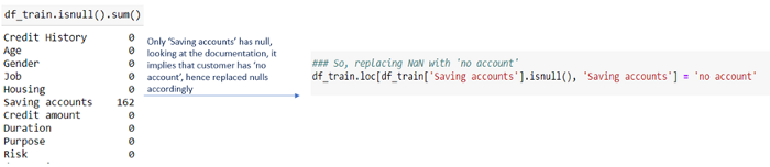
Another quick look at the data summary tells us that ‘Saving Accounts’ has a category as Nan. Investigate what does Nan imply -missing value or a genuine data entry. Here, ‘Nan’ entry corresponds to ‘No savings account’.
Checking the training and test data distribution:
• One of the most critical assumption in ML data modelling is that train and test dataset belong to similar distribution, as is evident from graphs below. Note that the train data is used as a reference to estimate the future credit worthiness of customers, hence the ML solution is probabilistic and not guaranteed based on past data. This emphasizes the property of generalization of ML solution
K-S statistic is a numeric measure to check the null hypothesis of whether the 2 distributions are identical. A K-S statistic value smaller than the p value suggests that we cannot reject the null hypothesis that the two distributions are same.

K-S Statistic


‘Age’ variable

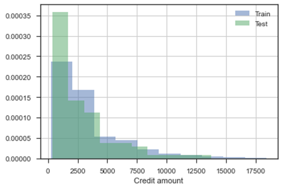
‘Credit amount’
Blue color histogram is from Train data and Green color is from Test data, the histogram plots from two distribution are sharing significant overlap with each other implying no significant drift (or in other words, they are drawn from similar distribution).
Exploratory data analysis:
Let’s look at how many missing records are there:

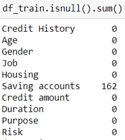
Null values
Only ‘Saving accounts’ variable has Nan entries, our initial dig at data comes handy here and we are able to handle these Nan by replacing them with another category — ‘no account’.
Also, try creative and innovative ways of presenting the analysis while writing a report, it is highly possible that the report might goes through a wide genre of audience (stakeholders).
As we might not know the end user of the report in advance, it is good to explain the ML solution workflow in as simple terms as possible while not losing the core analysis.
For this, I try following:
Setting up the right context in the initial slides so that there are no gaps.
Gradually, increase the level of complexity (aka technical details), as you progress through the report.
It has twofold benefits — the reader feels confident with the relatively fewer complex details in initial slides and is able to pick the relevant information from the forthcoming slides based on the primary understanding.
Also, try to aid the analysis with as much visualization as possible.
Ways to put the analysis in the report
The key focus should be writing a concise report while not leaving out any technical details.
Assumptions:
There will always come a point in your analysis, where you need to take a call to make some assumptions appropriate for ML modelling.
Always highlight those with the rationale behind such assumptions. It becomes more approving if it echoes business consent as well.
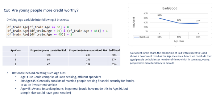
For example, we want to check if younger people are more credit worthy. One possible approach is to bin the variable ‘Age’ into 3 categories, as shown below. Providing the rationale from ML modelling standpoint also gives business a sneak peek into their data from technical perspective.
Here, I chose 45 years to mark the cut-off for 2nd bin, could have very well made it 50 (as 50 sounds more reasonable to assume the loan-averse category of people) but the trend analysis would not have had decent sample size to draw the conclusion. So, I preferred to take the middle ground and took 45 years as the age cut off to categorize the variable.

Snapshot of EDA in the report
Cross validation:
Canonically, dependencies learnt from the training data are checked on validation data to select the model based on a pre-decided evaluation metric. The selected model is then deployed to make predictions on test data. Cross-validation divides the training data iteratively into multiple folds and keeps one-fold aside for validation, I am using 5-fold CV in the analysis.
Decide the evaluation metric:
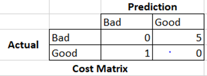
It carries huge significance and needs discussion with business at the beginning. For example, in credit risk prediction, the business ask is to give more penalty on the predictions if a customer is classified as Good risk, when in fact they bring Bad risk.
The cost matrix for the business case looks like below:
Give a background of where you are coming from, what all metrics are suitable for this problem:
F score is generally used as evaluation metric when there is no preference between Recall and Precision: 2PR/(P+R), where
P: Precision: focus on reducing False Positives (FP)
R: Recall: focus on reducing False Negatives (FN)
After the context setting, explain the final evaluation metric you narrow down to and reason behind such selection. I am using F beta score as an evaluation metric where beta suggests the weight on Recall. F1 score is same as F beta score with beta = 1.
As discussed above, there is a cost on classifying the customer as Good Risk when they are Bad Risk, i.e. predicting Good Risk (class 1, positive class) when it is False i.e. False Positives (FP) draws heavy penalty based on our business objective
Precision = TP/(TP+FP), so our goal is to prioritize Precision which translates to reducing the FP. So, we need to put more weight on Precision which is achieved from beta < 1.
Feel free to give some extra knowledge (it doesn’t hurt) which might not have come from business but is worthy to be put across the table.
Had the objective been to give penalty on predicting Bad risk when they are Good Risk, then based on such ML recommendations, we will be able to save potential business loss from refrained lending.
In that case, the focus would be on False Negatives (FN) i.e. you are predicting Bad Risk (class 0, negative class) while the customer was in Good Risk category. So, we predicted negative which went wrong implying more emphasis should be on reducing FN, which in turn would lead to more weight on Recall (TP/TP+FN)
Pipeline Flow:
It is considered good to visually present the summary of all the steps you have taken — right from the raw input data passing through data-processing pipeline to model selection to predictions. This step to tie-together all the components is my personal favourite, as it brings a level of abstraction as well as gives a clear picture of what was done to accomplish the end predictions

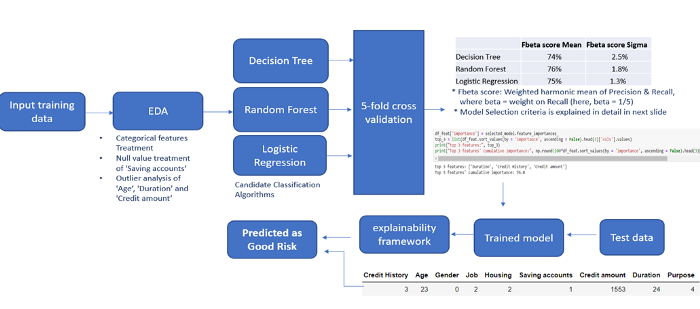
ML pipeline flow
Explaining the predictions:
Finally, it all comes down to how you explain the predictions. After giving a background to the model ‘Interpretability framework” you are choosing, give a description explaining the ‘Whys’:

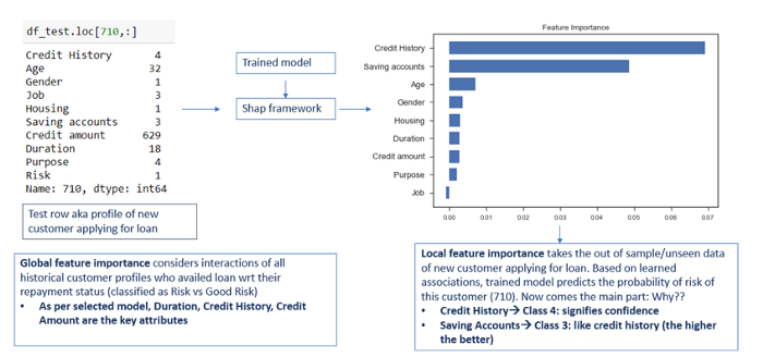
Model Interpretability
Note that there is no one way of approaching an ML solution and so, even report making, this was my way of presenting the solution. Hope it is of some value to you.
Would love to connect to the readers to learn from their experience — the better and effective ways of communicating results and approach.
Source: Paper.li


Comments