Go and CPU Caches
- The Tech Platform

- Jun 2, 2020
- 7 min read
According to Jackie Stewart, a three-time world champion F1 driver, having an understanding of how a car works made him a better pilot.
“You don’t have to be an engineer to be a racing driver, but you do have to have Mechanical Sympathy”
Martin Thompson (the designer of the LMAX Disruptor) applied the concept of mechanical sympathy to programming. In a nutshell, understanding the underlying hardware should make us a better developer when it comes to designing algorithms, data structures, etc.
In this post, we will dig into the processor and see how understanding some of its concepts can help us when it comes to optimizing solutions.
Fundamentals
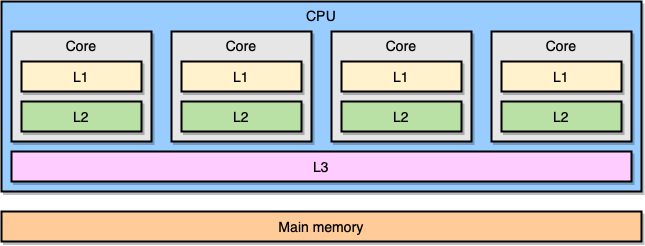
Modern processors are based on the concept of symmetric multiprocessing (SMP). In a SMP system, the processor is designed so that two or more cores are connected to a shared memory (also called main memory or RAM). Also, to speed up memory accesses, the processor has different levels of cache called L1, L2 and L3. The exact architecture may vary depending on the provider, the processor model, etc. Yet, the most frequent model is to have L1 and L2 local to a core and L3 shared across all cores:
SMP Architecture
The closer a cache is to a CPU core the smaller is its access latency and size:
Again, these exact figures depend on the processor model. Yet, to get a rough estimate: if we consider that accessing the main memory takes 60 ns, accessing L1 is about 50 times faster.
In the world of processors, there is an important concept called locality of reference. When a processor accesses to a particular memory location, it is very likely that:
It will access the same location in the near future: this is the temporal locality principle.
It will access memory locations nearby: this is the spatial locality principle.
Temporal locality is one of the reasons to have CPU caches. Yet, how do we leverage spatial locality? Instead of copying a single memory location to the CPU caches, the solution is to copy a cache line. A cache line is a contiguous segment of memory.
The size of a cache line depends on the cache level (and again of the processor model). For example, here is the size of the L1 cache line on my machine:
$ sysctl -a | grep cacheline
hw.cachelinesize: 64
Instead of copying a single variable to the L1 cache, the processor will copy a contiguous segment of 64 bytes. For example, instead of copying a single int64 element of a Go slice, it will copy this element plus the seven int64 elements as well.
A Concrete Application of Cache Lines in Go
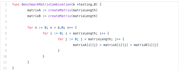
Let’s see a concrete example that will show us the benefits of CPU caches. In the following code, we will combine two squared matrices of int64 elements:
Given matrixLength set to 64k, it leads to the following result:
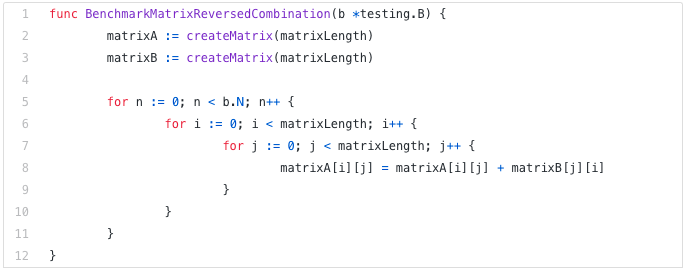
BenchmarkMatrixSimpleCombination-64000 8 130724158 ns/opNow, instead of adding matrixB[i][j] we will add matrixB[j][i]:
Does it impact the results?
BenchmarkMatrixCombination-64000                           8  130724158 ns/op
BenchmarkMatrixReversedCombination-64000                   2  573121540 ns/op
Quite drastically! How can we explain it?
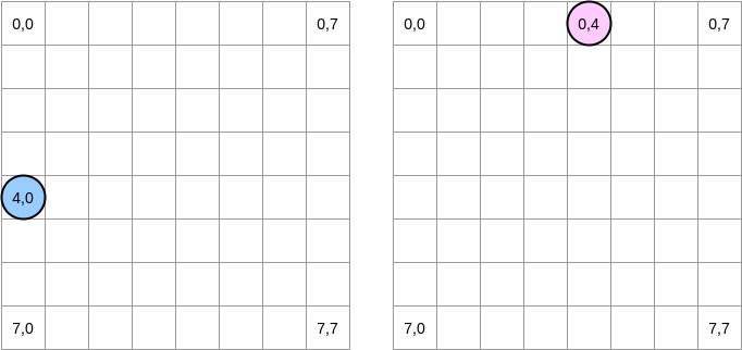
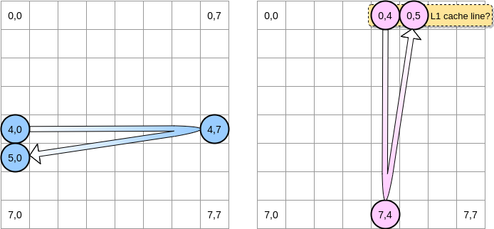
Let’s try to draw what’s happening. The blue circle is a pointer on the first matrix and the pink one on the second matrix. As we have to set matrixA[i][j] = matrixA[i][j] + matrixB[j][i], when the blue pointer is at position (4,0), the pink one is at position (0,4):
In this diagram, we represent the matrices with absciss and ordinate and the (0,0) position being the top left square. In memory, all the different rows of a matrix are allocated contiguously. Yet, for the sake of clarity, let’s stick with a mathematical representation. Moreover, in the following examples the matrix size is a multiple of the cache line size. Hence, a cache line will not “overtake” on the next row.
How do we iterate on both matrices? The blue pointer moves to the right until it reaches the last column and then it moves to the next row at position (5,0), etc. Conversely, the pink pointer moves downwards and then goes to the next column.
When the pink pointer accesses to the position (0,4), the processor will cache the whole line (in our example, the cache line size is 4 elements). Therefore, when the pink pointer reaches position (0,5), we may assume that the variable is already present in L1, isn’t it?
The answer depends on the matrix size:
If the matrix is small enough compared to the size of L1, then yes, the element (0,5) will already be cached.
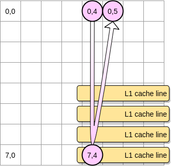
Otherwise, the cache line will be evicted from L1 before the pointer reaches position (0,5). Therefore, it will generate a cache miss and the processor will have to access the variable differently (using L2 for example). We would be in a state like this:
How small should the matrix be to benefit from L1? Let’s do some math. First, we need to know what is the L1 cache size:
$ sysctl hw.l1dcachesize
hw.l1icachesize: 32768
On my machine, the L1 cache is 32768 bytes whereas the L1 cache line is 64 bytes. Therefore, I can store up to 512 cache lines on L1. What if we run the same benchmark with a matrix composed of 512 elements?
BenchmarkMatrixCombination-512                1404     718594 ns/op
BenchmarkMatrixReversedCombination-512        1363     850141 ns/opp
Though we closed the gap (with a 64k matrix it was ~300% slower), we can still notice a slight difference. What could be wrong? In the benchmarks, we work on two matrices. Hence, the CPU has to store cache lines for both. In a perfect world (without other applications running, etc.), the L1 cache is 50% full because of the first matrix and 50% full because of the second one. What if we divide again by 2 the matrix size to work on 256 elements:
BenchmarkMatrixCombination-256                5712     176415 ns/op
BenchmarkMatrixReversedCombination-256        6470     164720 ns/op
Now we finally reached a point where the two results are (almost) equivalent.
Why is the second benchmark slightly faster than the first one? The difference looks to be quite subtle and related to the assembly code produced by Go. In the second case, the pointer on the second matrix is managed differently using an LEA (Load Effective Address) instruction. When a processor needs to access a memory location, there is a translation from the virtual to the physical memory. Using LEA allows computing a memory address without having to go through this translation. For example, if we manage a slice of int64 elements and that we already have a pointer on the first element address, we can use LEA to load the second element address by simply shifting the pointer to 8 bytes. In our example, it might be a potential reason why the second test is faster. Yet, I’m not an assembly expert so feel free to challenge this analysis. I uploaded the assembly code of the first function and the second one (reverse) if you want to take a look.
Now, how can we limit the impacts of the processor cache miss in the case of a larger matrix? There is a technique called loop nest optimization. We have to iterate only within a given block to benefit from cache lines as much as possible.
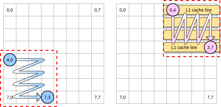
Let’s define in our example a block as a square of 4 elements. On the first matrix, we iterate from (4,0) to (4,3). Then we switch to the next row. Hence, we only iterate on the second matrix from (0,4) to (3,4) before to switch to the next column.
When the pink pointer iterates over the first column, the processor will store the corresponding cache line. Therefore, iterating over the rest of the block means to benefit from L1:
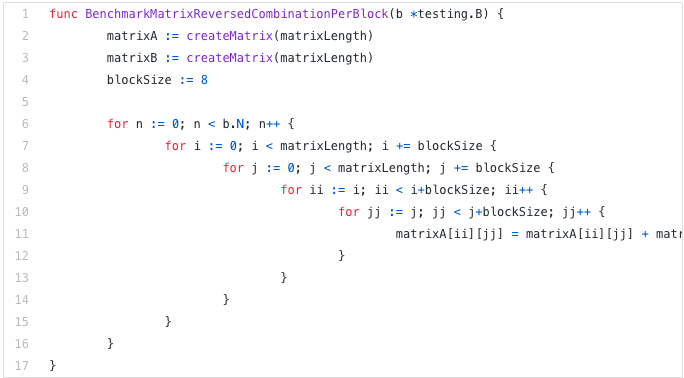
Let’s write the Go implementation of this algorithm but first, we have to choose the block size carefully. In the previous example, it was equal to the cache line. It should not be smaller, otherwise, we will store elements that will not be accessed. In our Go benchmark, we store int64 elements (8 bytes). The cache line is 64 bytes so it can store 8 elements. Then, the block size value should be at least 8:
Our implementation is now more than 67% faster than when we were iterating through the whole row/column:
BenchmarkMatrixReversedCombination-64000          2  573121540 ns/op
BenchmarkMatrixReversedCombinationPerBlock-64000  6  185375690 ns/op
This was a first example to demonstrate that understanding how CPU caches are working can potentially help us in designing more efficient algorithms.
False Sharing
We should now have a good understanding of how the processor manages its internal caches. As a quick recap:
Because of the spatial locality principle, the processor does not put a simple memory address but a cache line.
The L1 cache is local to a given CPU core.
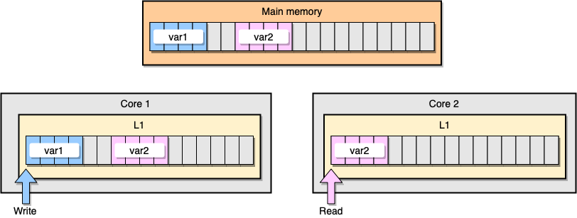
Now, let’s discuss the L1 cache coherency with an example. Two variables var1 and var2 are stored in the main memory. One thread on one core accesses to var1 whereas another thread on another core accesses to var2. Assuming that both variables are contiguous (or almost), we end up in a situation where var2 is present in both caches:
L1 cache example
What happens if the first thread updates its cache line? It could potentially update any location of its line including var2. Then, when the second thread reads var2, the value may not be consistent anymore.
How does a processor maintain cache coherency? If two cache lines share some common addresses, the processor will mark them as Shared. If one thread modifies a Shared line, it will mark both as Modified. To guarantee caches coherency, it requires coordination between the cores which may significantly degrade the application performance. This problem is called false sharing.
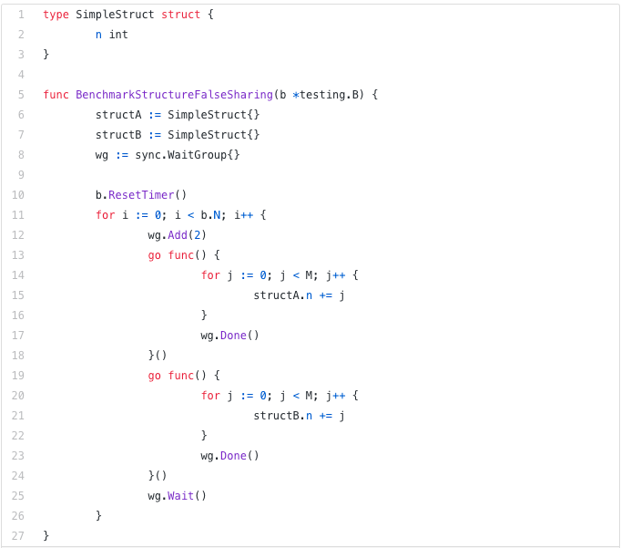
Let’s see a concrete application in Go. In this example, we instantiate two structures one after the other. Hence, these structures should be allocated contiguously in memory. Then, we create two goroutines where each one accessing its structure (M is a constant equal to 1 million):
In this example, the variable n of the second structure is accessed only by the second goroutine. Yet, as the structures are contiguous in memory, it will be present in both cache lines (assuming that both goroutines are scheduled on threads living on separate cores which is not necessarily the case). Here is the benchmark result:
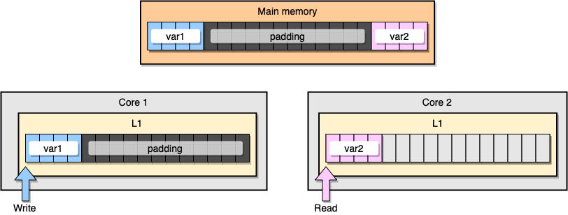
BenchmarkStructureFalseSharing 514 2641990 ns/opHow can we prevent false sharing? One solution is to use memory padding. The goal is to make sure that there is enough space between the two variables so that they belong to different cache lines.
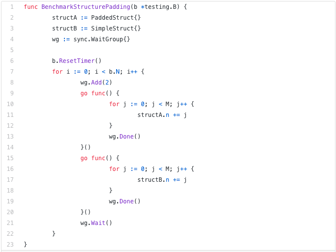
First, let’s create an alternative to the previous structure by padding the memory after the variable declaration:
Then, we instantiate the two structures and we keep accessing the two variables in separate goroutines:
Memory-wise, this example should look like this with the two variables being part of different cache lines:
Memory padding
Let’s see the results:
BenchmarkStructureFalseSharing         514    2641990 ns/op
BenchmarkStructurePadding              735    1622886 ns/op
Our second example using padding is about 40% faster than our initial implementation 🎉. There is a tradeoff though. To speed up the time execution, the memory padding requires to allocate more memory.
Mechanical sympathy is an important concept when it comes to application optimization. In this post, we have seen examples showing that understanding how CPU processors are working helped us in reducing execution time.
Source: paper.li

















Comments