
A Real-World Use Case for NLP, Leveraging T5 and PyTorch Lightning and AWS SageMaker

Natural language processing (NLP) is the technology we use to get computers to interact with text data. Popular applications include chat bots, language translation and grammar correction. Traditionally, it’s a field dominated by word-counting techniques like Bag-of-Words (BOW) and Term Frequency-Inverse Document Frequency (TF-IDF), where the goal is to make inferences based on the words present in the data. However, with recent breakthroughs in deep learning, we’re seeing the possibilities in NLP explode.
The Self-Attention Mechanism
Cornell University’s “Attention Is All You Need,” arguably the most influential NLP paper published in the last five years, introduced the “self-attention mechanism.” This mechanism created a simple solution to the problems the top NLP machine learning models were facing. At that time, the state-of-the-art NLP models were sequence-to-sequence (seq2seq) Recurrent Neural Networks (RNN), which performed well on short text strings but struggled mightily when used on long-blocks of text. They were also very costly to train. Self-attention replaced recurrence, since it was simpler to calculate and expanded the length of text that could be processed.
Possibly the biggest benefit of self-attention is how easily it scales. Multiple layers of self-attention can be ensembled together and calculated at once in what’s known as the “multi-headed attention mechanism” — the core of present-day machine learning in NLP.
BERT And Pals
Maybe the most famous deep-learning model to be released, Bidirectional Encoder Representations from Transformers (BERT) is a seq2seq model comprised of transformer blocks. These transformers are just a collection of multi-headed attention layers ensembled together. The release of BERT started a revolution in NLP, similar to the one in the deep learning computer vision space in the 2010s. BERT showed the possible applications of these transformer models in almost every NLP task, including classification, named-entity recognition and sentiment analysis.
Since BERT, we’ve seen an unending supply of new transformer models, with each one surpassing the previous on at least one NLP task. In this article, we’ll focus on building a conversation summarization model using T5. I highly encourage you to continue researching fascinating models like RoBERTa from FacebookAI and GPT-3 from OpenAI.
Summarizing Conversations Walkthrough
Today, everyone is communicating more than ever. Between social media, text messages and email, it can be difficult to keep up and ignore the noise. To remedy this, I’ll use T5 to create a model that will summarize conversations.
I’ll do so by leveraging the following technologies:
AWS SageMaker
AWS S3
AWS CloudWatch
PyTorch
Pytorch-Lightning
HuggingFace/Transformers
Preparing The Dataset
Obtaining a proper dataset is one of the hardest tasks in modern NLP machine learning problems, as it often involves very time-intensive manual labelling and, in our case, by-hand summarization. Fortunately, the models I’ll share thrive on “transfer learning,” which is the process of training a model on one dataset, then later training again on another. The latter is often referred to as “fine tuning.”
To begin, I’ll first train my model on the SAMSum Corpus Dataset, a dataset of more than 16,000 conversations between two people, which has already been summarized by humans.
Listing 1: Example Data Point
{
    'id: '13818513',
    'summary': 'AmandabakedcookiesandwillbringJerrysometomorrow.',
    'dialogue': "Amanda: I baked  cokies. do you want some?\r\nJerry: Sure!\r\nAmanda: I'll bring you tomorrow :-)"
}
Luckily, this dataset is broken down into train, test and validation sets. On top of that, the text within the datasets is very clean. To quickly perform exploratory data analysis (EDA) on this dataset, I’ll join the three sets into one. Later, I’ll shuffle them and split them back into three.
Often in NLP, you’ll spend much more time massaging your text data, but as you can see in Listing 2, I’m only going to remove the “\r” and “\n” characters.
Listing 2: Processing Raw Data
import json
import pandas as pd
    val_path='../data/raw/val.json'
    test_path='../data/raw/test.json'
    train_path='../data/raw/train.json'

with open(val_path) as in_file:
    val=json.load(in_file)
    in_file.close()

with open(test_path) as in_file:
    test=json.load(in_file)
    in_file.close()

with open(train_path) as in_file:
    train=json.load(in_file)
    in_file.close()

data=train + test+val
assert len (data) ==len(train) + len(test) + len(val)

df=pd.DataFrame(data)
df['dialogue'] =df['dialogue'].str.replace('\r', '')
df['dialogue'] =df['dialogue'].str.replace('\n', '')
df['summary'] =df['summary'].str.replace('\r', '')
df['summary'] =df['summary'].str.replace('\n', '')
As you can see in Listing 3, this leaves us with one DataFrame in the form of:
Listing 3: Processed Data Sample

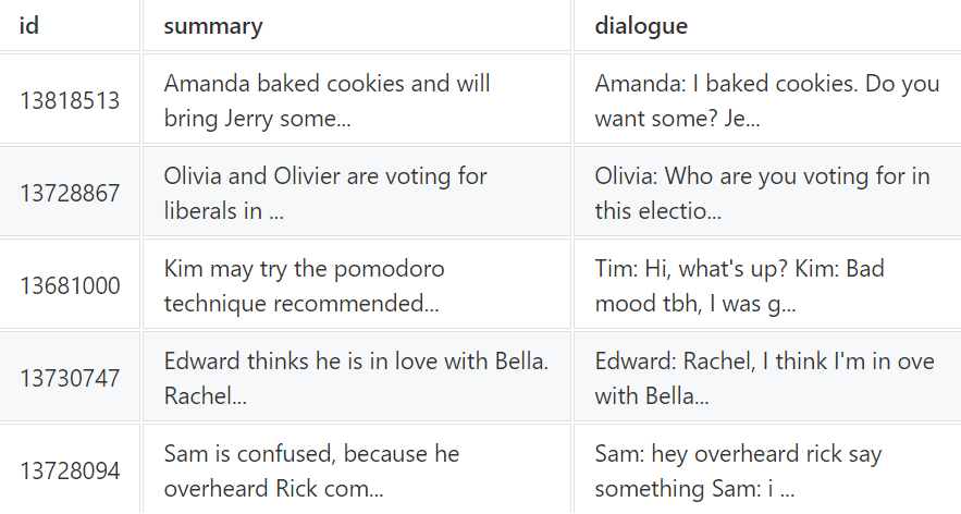
The most apparent downside to using transformer-based models like T5 is the input sequence length limitation. T5 has a maximum sequence length of 512 tokens. This means I must choose between either truncating my input dialogues down to the limit or only using data points where the dialogue is below the threshold. First, I’ll tokenize the data and then explore the distribution of the sequence lengths.
To tokenize the data, I’ll use the transformers library from HuggingFace. This is a fantastic library that allows you to easily interact with the latest pretrained-models in NLP for specific use cases.
from transformers import T5Tokenizer
    t5_tokenizer = T5Tokenizer.from_pretrained('t5-small')
Next, I’ll gather the dialogues and summaries into lists of strings and pass them through the new tokenizer. Because I’m using T5, I need to prepend each dialogue with summarize:. This ensures T5 knows which modeling task to perform.
Listing 4: Tokenizing The Data
dialogue=df['dialogue'].values.tolist()
summary=df['summary'].values.tolist()
data=t5_tokenizer.prepare_seq2seq_batch(
    src_texts=[f'summarize: {d}] ford in dialogue],
    tgt_texts=summary,
    padding='max_length',
    truncation = True,
    return_tensors ='pt'
)
For more information on all of the different tasks T5 is capable of, I highly recommend reading this blog post from Google AI.
In this command I’m doing a ton of neat things:
Tokenizing the data from strings into sequences of integers
Applying padding to all the data points that are shorter than the Maximum Sequence Length of 512 tokens
Truncating any longer sequences down to 512 tokens
Creating an attention mask
Returning PyTorch tensors
After the tokenization, I have a dictionary-like object that contains input_ids, which are tokenized dialogues. As well as attention_mask, which is a key of sorts that tells our model where we have padded the sequence. This helps us accurately compute accuracy and loss later. Lastly, it also contains labels, which are tokenized summaries.
Now that I have my tokens, I can explore how long they are.

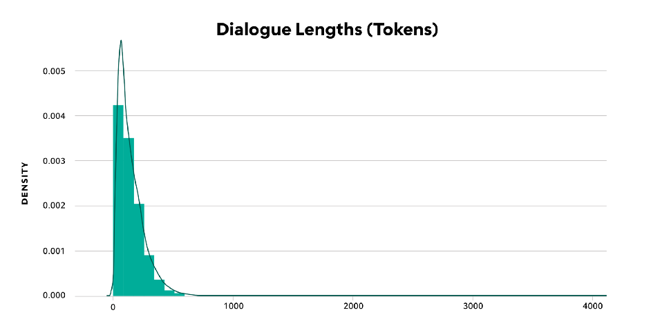
Figure 1 — Dialogue Lengths (Tokens)


Figure 2 — Summary Lengths (Tokens)
In Figure 1, most of the data falls below 512 tokens, but the dataset contains a few samples with more than 4,000 tokens. I’ll drop these longer sequences and continue.
In Figure 2, most of my dialogues fall at or below the 512 token length, and my summaries are well under that limit. So, I’ll simply truncate any sequences that are longer than the maximum length and proceed.

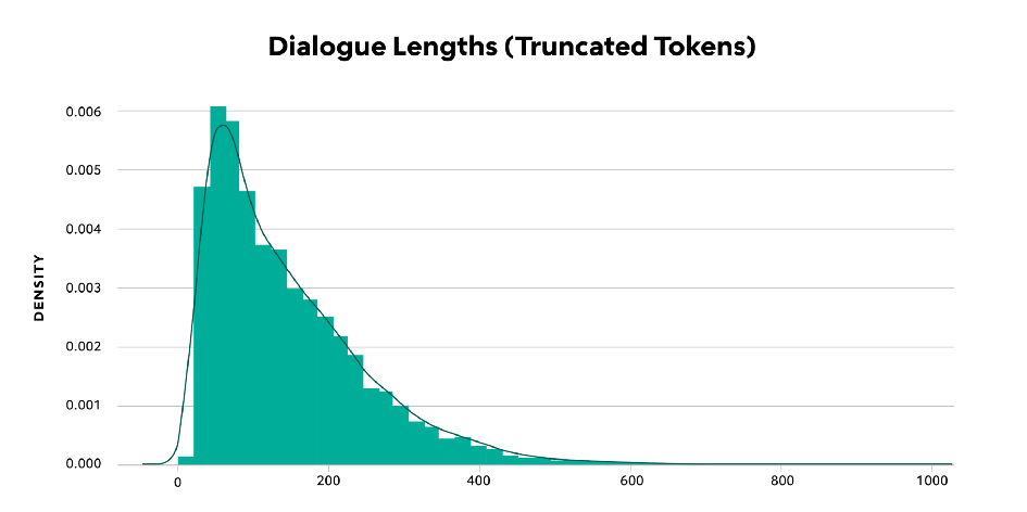
Figure 3 — Dialogue Lengths (Truncated Tokens)

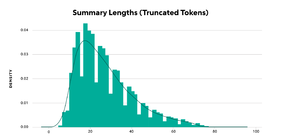
Figure 4 — Summary Lengths (Truncated Tokens)
I encourage you to perform additional EDA on this dataset, but for the purpose of brevity, I’ll call it done for now and move onto creating and splitting my data into train, test and validation sets.
Creating And Splitting A Dataset
First, I create a TensorDataset from our tokenized tensors, as shown in Listing 5.
Listing 5: Creating PyTorch Tensor Dataset
from torch.utils.data import TensorDataset

tdata=TensorDataset(
    data['input_ids'],
    data['attention_mask'],
    data['labels']
)
Next, I want to use 80% of my data for training, 10% for validation and reserve the remaining 10% for final testing. As shown in Listing 6, I’ll calculate the sizes of each split, then use the random_split() function to create those splits. Finally, I’ll save these three datasets.
Listing 6: Creating Training, Testing, & Validation Datasets
import torch
from torch.utils.data import random_split
    train_size = int(data['input_ids'].shape[0] *0.80)
    test_size = int(data['input_ids'].shape[0] *0.10)
    val_size = int(data['input_ids'].shape[0]) -train_size-test_size

assert train_size+test_size+val_size == int(data['input_ids'].shape[0])

train, test, val=random_split(
    dataset=tdata,
    lengths=(train_size, test_size, val_size)
)

torch.save(train, '../data/processed/t5_train_dataset.pt')
torch.save(test, '../data/processed/t5_test_dataset.pt')
torch.save(val, '../data/processed/t5_val_dataset.pt')
Lastly, I’ll upload these files into an S3 bucket. If you’ve never created one before or would like a refresher, I recommend checking out the official documentation from AWS.
Training The Model
Over the past year or so, I’ve become a huge fan of PyTorch-Lightning, a python library based on PyTorch, which aims to help you make your code more readable and reproducible. In this section, I’ll utilize this library to train the T5 model for conversational summarization. I’ll explain what’s happening at a high level, but I won’t be able to go in-depth on the inner workings of PyTorch-Lightning. If you’re interested in a deeper tutorial, drop a comment down below.
For my purpose, I’ll create a lightning module around the T5ForConditionalGeneration model provided by HuggingFace, as shown in Listing 7.
Listing 7: Defining The PyTorch-Lightning Module
import torch
from torch.utils.data import DataLoader
from torch.optim.lr_scheduler
import LambdaLR import pytorch_lightning as pl
from transformers import T5ForConditionalGeneration, T5Tokenizer, get_cosine_schedule_with_warmup

classT5LightningModule(pl.LightningModule):
    def__init__(
        self,
        pretrained_nlp_model: str,
        train_dataset: str,
        test_dataset: str,
        val_dataset: str,
        batch_size: int,
        learning_rate: float=3e-05
    ):
        super().__init__()

        self.batch_size=batch_size
        self.train_dataset=train_dataset
        self.test_dataset=test_dataset
        self.val_dataset=val_dataset
        self.hparams.learning_rate=learning_rate
      self.t5=T5ForConditionalGeneration.from_pretrained(pretrained_nlp_model)

self.tokenizer=T5Tokenizer.from_pretrained(pretrained_nlp_model)
To start building our SageMaker training job, in Listing 8, we begin by defining:
metric_definitions These are regular expression patterns that AWS CloudWatch will scrape and track. This is a quick-and-dirty method for monitoring model training if you don’t want to integrate with TensorBoard, Comet or WandB.
start_time This is just a timestamp. Training jobs must be unique, so I simply append the start_time to my training job name.
hparams Here I define any parameters that I want to pass to my lightning module during training.
Listing 8: Setting Metric Definitions And Hyperparameters In AWS SageMaker
import time

metric_definitions= [
    {'Name': 'train:loss', 'Regex': 'train_loss: (.*?);'},
    {'Name': 'validation:loss', 'Regex': 'val_loss: (.*?);'},
    {'Name': 'test:loss', 'Regex': 'test_loss: (.*?);'},
    {'Name': 'current_epoch', 'Regex': 'current_epoch: (.*?);'},
    {'Name': 'global_step', 'Regex': 'global_step: (.*?);'}
]

start_time=time.strftime('%Y%m%dT%H%M%S')

hparams= {
    'batch-size': 8,
    'learning-rate': 3e-05,
    'model-path': 't5-small',
    'job-name': f
    't5-small-{start_time}',
    'epochs': 25,
    'gpus': 1
}
TensorBoard Logging
To enable live logging with TensorBoard, I need to do two things. First, I’ll create a TensorBoardOutputConfig module. This object will be responsible for moving my TensorBoard logs from the Docker container that my code is running in to the S3 bucket. Listing 9: Defining TensorBoard SageMaker Object
from sagemaker.debugger import TensorBoardOutputConfig

tensorboard_output_config = TensorBoardOutputConfig(
    s3_output_path=f'{bucket}/tb_logs',
    container_local_output_path='/opt/tb_logs')
I also need to create a TensorBoardLogger. This object will generate the TensorBoard logs.
Listing 10: Defining TensorBoard PyTorch Lightning Logger
from pytorch_lightning.loggers import TensorBoardLogger
tb_logger = TensorBoardLogger(save_dir='/opt/tb_logs', name=args.job_name)
Now I can use the self.log() anywhere in my lightning module and have those in the S3 bucket in almost real time.
Early Stopping
Early stopping is a great technique for cutting down on training costs while preventing overfitting. Luckily, PyTorch Lightning makes it extremely easy.
In Listing 11, I define an EarlyStopping object that will monitor validation loss. If the validation loss doesn’t decrease by more than the min_delta within three epochs, this module will stop the training.
Listing 11: Defining An EarlyStopping Object
from pytorch_lightning.callbacks.early_stoppingimportEarlyStopping

early_stop = EarlyStopping(
    monitor='val_loss',
    # the metric to watch for changes.

    min_delta=0.01,
    # the minimum change to be considered a change.

    patience=3,
    # the number of epochs to pass without a min_delta change before
    stopping.

    mode='min'
    # the direction we aim for the monitor metric to move in.
 )
Monitoring Learning Rate
In this training job, I use a custom learning rate schedule, shown in Listing 12, which increases the rate over the first 500 steps, then decreases it over the next 20,000.
Listing 12: Defining A Learning Rate Schedule
# Inside our T5LightningModule
    def configure_optimizers(self):
        optimizer=torch.optim.Adam(
            self.parameters(),
            lr=self.hparams.learning_rate,
            weight_decay=0.01,
            betas=(0.9, 0.999),
            eps=1e-08
)
         scheduler=get_cosine_schedule_with_warmup(
              optimizer,
              num_warmup_steps=500,
              num_training_steps=20000
)
         gen_sched= {'scheduler': scheduler, 'interval': 'step'}

         return [optimizer], [gen_sched]
It would be great if I could track those changes over time. Yet again, PyTorch-Lightning comes in clutch! In Listing 13, you can see how to track the learning rate over time.
Listing 13: Defining Learning Rate Monitor
from pytorch_lightning.callbacks import LearningRateMonitor

lr_logger = LearningRateMonitor(logging_interval='step')
Easy as that! Now, I have my learning rate logged.
Model Checkpointing
Model checkpointing, shown in Listing 14, is an extremely important feature that enables us to keep our best-performing snapshot of our model at any given time.
Listing 14: Defining Model Checkpointing Object
from pytorch_lightning.callbacks.model_checkpoint import ModelCheckpoint

model_checkpoint=ModelCheckpoint(
    filepath=args.model_dir,
    monitor='val_loss',
    mode='min',
    save_top_k=1
)
Distributed Training
One of the key features needed when training deep learning models, and especially these really large NLP models, is distributed training across multiple GPUs and even multiple nodes. I’m sure by now you know what’s coming: PyTorch Lightning makes this incredibly easy. I simply add the distributed_backend=“ddp” argument to the trainer, and everything else is handled for me.
Trainer
The last thing I need to do is build the Lightning Trainer. In Listing 15, I combine all the previous steps into one module and begin to train the model.
Listing 15: Defining Trainer Parameters
# in our training loop

    trainer_params= {
        'max_epochs': int(args.epochs),
        'default_root_dir': args.output_data_dir,
        'gpus': int(args.gpus),
        'logger': tb_logger,
        'early_stop_callback': early_stop,
        'checkpoint_callback': model_checkpoint,
        'callbacks': [lr_logger]
    }

    if trainer_params['gpus'] >1:
        trainer_params['distributed_backend'] ='ddp'

    trainer=pl.Trainer(**trainer_params)
    trainer.fit(model)
AWS SageMaker
The easiest way to work with SageMaker is by creating a command line interface using the argparse library. If you’ve never done so before, I highly recommend checking out this tutorial from RealPython.com.
Interacting via a command-line allows for numerous benefits, the most apparent being the ability to pass variables from the hparams object to the training job. Now if you’ve never worked with SageMaker before, there are some nuances to working in it. The first is how it expects to receive data. SageMaker expects data to be in the following locations:
SM_CHANNEL_TRAIN — Training Data
SM_CHANNEL_TEST — Test Data
SM_CHANNEL_VAL — Validation Data
Also, SageMaker will upload the following directories to your specified S3 bucket after the training job completes.
This is where you should save your model artifacts: /opt/ml/model — s3://BUCKET/models
This is where you should store any other artifacts: /opt/ml/output — s3://BUCKET/output
To begin the training, I’ll create a PyTorch estimator object with all the SageMaker parameters I created earlier and then execute the training job.
Listing 16: Defining the SageMaker Estimator
from sagemaker.pytorch import PyTorch

estimator=PyTorch(
    entry_point='train_t5_model.py',
    source_dir='code',
    role=role,
    framework_version='1.6.0',
    instance_count=1,
    instance_type='ml.p3.2xlarge',
    output_path=s3_output_location,
    metric_definitions=metric_definitions,
    hyperparameters=hparams,
    tensorboard_output_config=tensorboard_output_config
)

estimator.fit({
    'train': f'{bucket}/data/processed/t5_train_dataset.pt',
    'test': f'{bucket}/data/processed/t5_test_dataset.pt',
    'val': f'{bucket}/data/processed/t5_val_dataset.pt',
})
I’m running the training on a ml.p3.2xlarge instance which contains 1 Tesla V100 GPU, the top-of-the-line hardware. If your training does not require a GPU, be sure to change this to something that fits your needs.
After the training begins, you can launch a TensorBoard application from your local computer using the command shown in Listing 17:
Listing 17: TensorBoard Dashboard
AWS_REGION={YOUR AWS REGION} tensorboard --logdir s3://{BUCKET}/tb_logsRunning the above code in my Terminal will launch TensorBoard on my local machine. However, it will begin to search for and pull logs from the S3 bucket that my SageMaker job is writing to. In Figure 5, you can see the three scalar-metrics that I’m logging: our train_loss, val_loss, test_loss, and learning_rate.

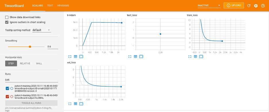
Figure 5 — TensorBoard Scalars
Because I’m doing a summarization task, I thought it would be handy to periodically generate model summaries and log those to TensorBoard. To see the code to do this, check out the validation_step method in the GitHub repository. In the below figure, you can see this output under the text tab in TensorBoard.

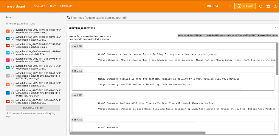
Figure 6 — Model Summaries Logged in TensorBoard
Deploying The Model
Now I have my model artifact in S3, so I can take it and deploy it any way I’m comfortable. SageMaker provides a quick and easy route, shown in Listing 18. I’ll need to create an inference.py file (look for an example in my GitHub repository). This will provide me with a REST API endpoint where I can begin using my model in production.
Listing 18: Deploying The Model Using AWS SageMaker
from sagemaker.pytorch.model import PyTorchModel

pytorch_model=PyTorchModel(
    model_data=f'{bucket}/models/model.tar.gz',
    role=role,
    source_dir='code',
    entry_point='inference.py',
    py_version='1.6.0',
    framework_version='1.6.0',
)

predictor=pytorch_model.deploy(
    instance_type='ml.c5.xlarge',
    initial_instance_count=1,
    endpoint_name='t5-small-con-sum'
)
Closing
The world of NLP has been flipped and turned upside down over the last few years. Every month or so, the big artificial intelligence researchers release a better model that we, as practitioners, can take advantage of in our day-to-day work. After reading this article, I hope you feel empowered to take these models into your own hands.
Source: Medium
The Tech Platform
Comments