
A SIMPLE, BEGINNER’S GUIDE TO MACHINE LEARNING ALGORITHMS
- The Tech Platform
- Sep 8, 2020
- 9 min read


The world today has witnessed some of the great successes of machine learning applications. We all have awed at the working of self-driving Google car and relied on online recommendation engines of Netflix and e-commerce sites. These are essentially based on state-of-the-art machine learning algorithms. Because of the advancements in computing technologies and exposure to huge amounts of data, the applicability of machine learning has dramatically increased.
The aim of machine learning is to make automated models such that they learn from data that is fed and produce reliable predictions and decisions without much human intervention. Although this technology is not new, the ability to apply complex mathematical calculations on big data has given a considerable momentum to this field in recent times.
According to the learning styles, machine learning techniques are broadly classified into – supervised, unsupervised, semi-supervised and reinforced learning. They are described here in brief.
1. Supervised learning – In this, a model is trained using a known set of input data with known responses to this data, also known as labeled data. The main categories of this kind of learning are- classification and regression.
• Classification– When the data is used to predict a category the data-point may belong to. For example, stating if an image is of an animal or a human. There can be two or more classifying categories.
• Regression– When the relationship between two variables needs to be defined and how the change in one variable affects the other, it becomes a regression model.
2. Unsupervised learning – A model is trained using unlabelled data where the model finds the structure on its own. Data is divided into clusters according to similarities and reducing the dimensionality makes complex data easy to analyze.
• Clustering– Grouping of variables into clusters according to some defined criteria. Further analysis is then performed in these clusters.
• Dimensionality Reduction– If the input data has high dimensionality, it becomes important to remove redundant, unwanted data.
3. Reinforcement learning– It is said to be the hope of true AI. The model learns how to interact with an environment and has a feedback mechanism such that it learns from its own experiences, through trial and error.
4. Semi-supervised learning– The model can be trained using both labeled and unlabelled data. It is supposed to learn the structure and also make predictions after organizing the data. Hence, it has some functionalities of both supervised and unsupervised learning.
This is a list of ML algorithms that come under the categories mentioned above. They do share similarities in terms of categorization, for example, an algorithm can be both neural network-based and instance-based at the same time. In this article, we explain the basic functioning of some of the commonly used algorithms and their broad applications. The list is not exhaustive in terms of algorithms or the groups they belong to but covers all the major types if one wants to decide what to use.
1. Decision Trees

It is a supervised learning technique where the model maximises the information gain and gives the best-suited decision based on all the possible outcomes. It uses a tree-like graphical representation where the branches signify the outcomes and leaf signify a particular class label- mostly, a Yes or a No to any outcome. This gives a structured way for businesses to make favorable decisions by assessing the probabilities. It is a fast performing algorithm that doesn’t use a lot of memory.
Decision trees are used for making classifications and predictions both. Hence, decision trees can be classification trees (binary or multiple categories) or regression trees (in case of continuous variables), although it does not fit well with continuous data as it produces classification plateaus.
Decision trees can be used when the data scientist wants to evaluate different operations of an alternate decision. The calculation path can be traversed back and forth to optimise decisions. It performs well even with erroneous or missing data and one of the main advantages is that the findings can be communicated and explained easily to anyone. It performs feature selection which makes it very useful for predictive analytics. Commonly used Decision Trees include
1. Classification and regression tree (CART)
2. C4.0 and C5.0
3. Conditional decision trees
2. Regression
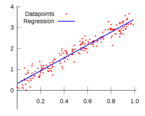
It is a statistical model that allows making predictions from data by understanding the relationship between a target variable and predictor variable (independent variable). There are several regression methods- linear and logistic regression being the most widely used. A curve or line is fit to the data points or variables and deviation of these data points from the curve is minimised. It helps the data scientists to predict the best set of variables for their model.
1. Linear regression – It is one of the most common technique in predictive modeling where two variables share a linear relationship, suggesting that it is sensitive to outliers. It is represented by the equation Y=a+bx+e, where e is the error term. The model can work on one or more predictor variables. To use Linear regression a data scientist may have to study the statistical parameters for minimising error.
2. Ordinary Least squares method (OLSM) – It is a method for performing Linear regression where the sum of the vertical distances of these points from the line is tried to be made as small as possible.
3. Logistic regression– This powerful statistic method is used for estimating discrete values-0 or 1 based on predictor variables. It uses a logarithmic function of the probabilities that maximises the log-likelihood rather than minimising mean error. It is widely used for classification problems. Regression methods are mostly used for risk assessment in financial or insurance domains. It is great for companies to predict sales, credit scoring and so on.
3. Bayesian Algorithms
These algorithms apply the Bayes theorem on conditional probability (P(A | B)) which performs classification on the assumption that the predictor variables do not depend on one another. It is one of the oldest concepts used in machine learning and till date it outperforms many sophisticated algorithms for classification. It is more suitable when the data sets are large and used widely in text-based applications.
It calculates the probability of a target variable belonging to a particular class having known a predictor value using the likelihood that this predictor belongs to the mentioned class and also knowing the individual probabilities of the class and the predictor.
The most popular Bayes algorithms are-
1. Naïve Bayes
2. Gaussian Naïve Bayes
3. Bayesian Belief Network
4. Multinomial Naïve Bayes
Some of the most famous uses of Bayes theorem are:
Sentiment analysis, Google’s pagerank algorithm, document classification technique for categorizing news articles, and spam emails classification
4. Support Vector Machines (SVM)
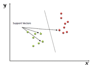
SVM is a supervised classifier that has proved to be more robust and effective compared to the probabilistic models. The data is plotted in an n-dimensional space, also called as a vector space where n is defined by the number of features defining a variable. The coordinates that define a data point is called its support vector. On plotting the data points, we divide the data points into groups by drawing a line (in case of two-dimensional data) or a hyperplane (in case of n-dimensional data) and perform classification. SVM tries to maximise the distance between various classes which allows it to perform better generalization.
In terms of diverse data, the classification cannot be performed using a hyperplane. Such SVMs are called non-linear SVMs. It uses a kernel such as Radial Basis Function (RBF) to map the non-linearly separable function into a higher dimension linearly separable function. SVM works efficiently on large vector spaces and gives better resistance against data overfitting. SVM is preferred when the target data is numeric such as in stock market analysis, image classification, etc.
5. Cluster Analysis

Clustering refers to segregation of similar data points into clusters according to predefined criteria. Either the data point completely belongs to a cluster or there is a probability associated with it being in the cluster. Clustering algorithms can be used prior to supervised technique to further improve the accuracy of results. Two of the main clustering algorithms widely used include:
1. K-means clustering – It is an unsupervised, iterative learning method where the dataset is divided into K number of clusters. On clustering, the algorithm calculates the centroid of each cluster and shifts a data point to a cluster depending on its proximity to its centroid. In every iteration, it calculates the local maxima until it reaches the point where no further shifting is required. K-median is also a clustering algorithm but not as widely used compared to K-means.
2. Hierarchical clustering– It uses a hierarchy of clusters which is represented using a dendrogram. Two nearest clusters are merged until there is only one cluster at the top of the representation. The decision of merging two closest neighbors is made on the basis of formulas. This algorithm cannot work on big data as easily as K-means does.
Application of clustering algorithms include:
Recommendation engines, search engines such as google, yahoo use it for clustering relevant webpages, internet security for finding anomalies and analysing social media trends.
6. Ensemble Algorithms

This technique combines prediction from a number of weaker algorithms by calculating averages or performing regression to make overall predictions. It gives an advantage that the model does not easily over-fit. However, combining results of several algorithms gives an error if bias and variance are found to be high or too low.
Some of the commonly used Ensemble methods are –
1. Bagging –Also called as Bootstrap Aggregating, it is a powerful statistical method where an estimated quantity such as mean or standard deviation of some values can be optimised. Bootstrapping refers to generating random samples with replacement. The data is divided into sub-samples on which calculations are performed and the result is then aggregated. This method successfully eliminates high variance which is found in decision trees. By using a number of decision trees and increasing the number of samples, overfitting is reduced.
2. Random forests – It is an improvement over bagging decision forest where some randomness is provided at the model level. In other words, each model is given slightly different data for training multiple times. The output of all the outcomes is combined and a final decision is made. It is used for both classifications and predictions.
3. Boosting – Boosting methods also produce multiple random samples, but mostly dependent on weights given to records in the previous sample which did not predict accurately – hence called weak learners. The final prediction is not a simple average of all the predictions, but a weighted average of them.
7. Dimension Reduction Techniques

Generally, it is not advised to feed a large number of features directly into a machine learning algorithm since some features may be irrelevant. The “intrinsic” dimensionality may be smaller than the number of features. In such cases algorithms like Principal Component Analysis (PCA), ICA (Independent Component Analysis), Singular Value Decomposition (SVD) and Linear discriminant analysis (LDA) are performed.
PCA– In this technique, variables are transformed into a new set of uncorrelated variables, which are a linear combination of original variables, known as principal components. The first principal component captures most of the possible variation of original data after which each succeeding component has the highest possible variance. The second principal component must be orthogonal to the first principal component. In other words, it does its best to capture the variance in the data that is not captured by the first principal component. PCA is an application of SVD. It is not suitable for use on noisy data.
In some cases, random forests, clustering, and decision trees are also used for successful dimension reduction. Dimension reduction has huge applications in computer vision and image processing. LDA with SVD is highly used in natural language processing tasks.
8. Instance-Based Algorithms
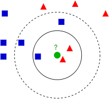
Instance-based algorithms take instances from the training data and compare new data to find similar instances and make predictions. K- nearest neighbors is a type of instance-based algorithm.
K-Nearest neighbors– It is an easy to understand algorithm for classification and regression. In this technique, predictions are made for an instance by finding the K most similar instances from the entire dataset. For finding the most similar instances, a distance formula known as Euclidian distance is used. Other popular distance formulae are Hamming distance, Manhattan and Minkowski distance, cosine distance, etc.
The value of K can be found by tuning the algorithm. Generally, a higher value of K is found to give better results. If K = 1, then the case is simply assigned to the class of its nearest neighbour. Choosing K turns out to be a challenge while performing KNN algorithm. KNN method is generally preferred when the data is less complex with low dimensionality.
KNN for regression is performed by calculating the median or mode of these K instances. Self-organizing maps (SOMs) and Linear Vector Quantization(LVQ) that are essentially Artificial Neural Network based algorithms can also be classified as Instance-based algorithms.
9. Artificial Neural Networks
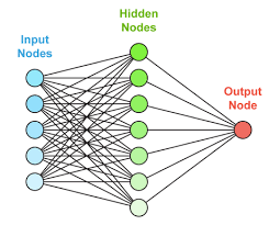
ANNs are models inspired from the human nervous system, that enables the network to learn by example and experience. It is used to find patterns in data to make predictions and perform classification. They are made of interconnected nodes arranged in three or more layers. These layers are input and output layer with one or more hidden layers.
There are certain traditional neural networks that separate it from deep learning algorithms. They are structurally less complex compared to deep learning networks. The input nodes take in data that is used to train the model. The output node gives an output after producing a weighted average of all these inputs. The weights are intuitively assigned at the hidden layer that changes adaptively with more iterations.
10. Deep Learning Techniques


With improvements in computation capabilities, deeper neural networks were developed. They are essentially perceptron networks but with a large number of hidden layers and nodes that facilitates better learning. They can work on very large datasets where the data is not labeled. It also eliminates the need for handcrafting features in pre-processing techniques.
The major types of DNNs include Convolutional Neural Network (CNNs), Recurrent Neural networks (RNNs), Recursive Neural Networks, etc.
Conclusion
As mentioned above, this was not an exhaustive list but these algorithms have found widespread usability and popularity among data scientists and analysts. For a beginner, it could be a daunting task to decipher which algorithms to choose for their applications. At times, even data scientists need to test their data on several algorithms to find the best match. Hence, a comprehensive knowledge of all these algorithms is important for helping businesses make the best possible use of these powerful tools.
Source: Paper.li