
Machine Learning Workflow on Diabetes Data : Part 02
- The Tech Platform

- Feb 18, 2021
- 6 min read


In my last article of this series, we discussed about the machine learning workflow on the diabetes data set. And discussed about topics such as data exploration, data cleaning, feature engineering basics and model selection process. You can find the previous article below.
Machine Learning Workflow on Diabetes Data : Part 01 After the model selection, we were able to identify that Logistic Regression performed better than the other selected classification models. In this article we will be discussing the next stages of the machine learning workflow, advanced feature engineering, and hyper parameter tuning.
Phase 5 — Feature Engineering (Revisited)
Not all the features need to be winners. Most of the time, there are features that don’t improve the model. Such cases can be found by further analysis of the features related to the model. “One highly predictive feature makes up for 10 duds”.
As mentioned in Phase 3, after model selection, Feature Engineering should be further discussed. Therefore we will be analyzing the selected model which is Logistic Regression, and how feature importance affects it.
Scikit Learn provided useful methods by which we can do feature selection and find out the importance of features which affect the model.
Univariate Feature Selection : Statistical tests can be used to select those features that have the strongest relationship with the output variable.
Recursive Feature Elimination : The Recursive Feature Elimination (or RFE) works by recursively removing attributes and building a model on those attributes that remain. It uses the model accuracy to identify which attributes (and combination of attributes) contribute the most to predicting the target attribute.
Principal Component Analysis : Principal Component Analysis (or PCA) uses linear algebra to transform the dataset into a compressed form. Generally this is called a data reduction technique. A property of PCA is that you can choose the number of dimensions or principal component in the transformed result.
Feature Importance : Bagged decision trees like Random Forest and Extra Trees can be used to estimate the importance of features.
In this tutorial we will be using Recursive Feature Elimination as the feature selection method.
First we import RFECV, which comes with inbuilt cross validation feature. Same as the classifier model, RFECV has the fit() method which accepts features and the response/target.
Logistic Regression — Feature Selection
from sklearn.feature_selection import RFECV
logreg_model = LogisticRegression()
rfecv = RFECV(estimator=logreg_model, step=1, cv=strat_k_fold, scoring='accuracy')
rfecv.fit(X, y)
After fitting, it exposes an attribute grid_scores_ which returns a list of accuracy scores for each of the features selected. We can use that to plot a graph to see the no of features which gives the maximum accuracy for the given model.
plt.figure()
plt.title('Logistic Regression CV score vs No of Features')
plt.xlabel("Number of features selected")
plt.ylabel("Cross validation score (nb of correct classifications)")
plt.plot(range(1, len(rfecv.grid_scores_) + 1), rfecv.grid_scores_)
plt.show()
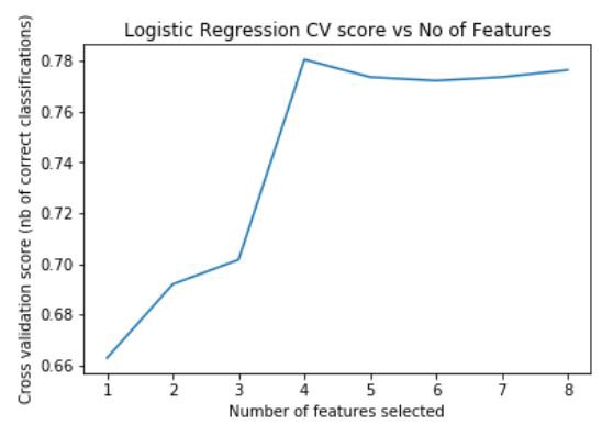
Fig — Feature importance of Logistic Regression
By looking at the plot we can see that inputting 4 features to the model gives the best accuracy score. RFECV exposes support_ which is another attribute to find out the features which contribute the most to predicting. In order to find out which features are selected we can use the following code.
feature_importance = list(zip(feature_names, rfecv.support_))
new_features = []
for key,value in enumerate(feature_importance):
    if(value[1]) == True:
        new_features.append(value[0])

print(new_features)
['Pregnancies', 'Glucose', 'BMI', 'DiabetesPedigreeFunction']
We can see that the given features are the most suitable for predicting the response class. We can do a comparison of the model with original features and the RFECV selected features to see if there is an improvement in the accuracy scores.
# Calculate accuracy scores
X_new = diabetes_mod[new_features]

initial_score = cross_val_score(logreg_model, X, y, cv=strat_k_fold, scoring='accuracy').mean()
print("Initial accuracy : {} ".format(initial_score))

fe_score = cross_val_score(logreg_model, X_new, y, cv=strat_k_fold, scoring='accuracy').mean()
print("Accuracy after Feature Selection : {} ".format(fe_score))
Initial accuracy : 0.7764400711728514 Accuracy after Feature Selection : 0.7805877119643279
By observing the accuracy there is a slight increase in the accuracy after feeding the selected features to the model.
Gradient Boosting — Feature Selection
We can also analyze the second best model we had which is Gradient Boost classifier, to see if features selection process increases the model accuracy and if it would be better than Logistic Regression after the process.
We follow the same procedure which we did for Logistic Regression
gb_model = GradientBoostingClassifier()

gb_rfecv = RFECV(estimator=gb_model, step=1, cv=strat_k_fold, scoring='accuracy')
gb_rfecv.fit(X, y)

plt.figure()
plt.title('Gradient Boost CV score vs No of Features')
plt.xlabel("Number of features selected")
plt.ylabel("Cross validation score (nb of correct classifications)")
plt.plot(range(1, len(gb_rfecv.grid_scores_) + 1), gb_rfecv.grid_scores_)
plt.show()
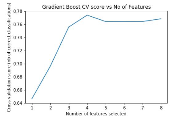
Fig — Feature importance of Gradient Boost
We can see that having 4 input features generates the maximum accuracy.
feature_importance = list(zip(feature_names, gb_rfecv.support_))
new_features = []
for key,value in enumerate(feature_importance):
    if(value[1]) == True:
        new_features.append(value[0])

print(new_features)
['Glucose', 'BMI', 'DiabetesPedigreeFunction', 'Age']
The above 4 features are most suitable for the model. We can compare the accuracy before and after feature selection.
X_new_gb = diabetes_mod[new_features]

initial_score = cross_val_score(gb_model, X, y, cv=strat_k_fold, scoring='accuracy').mean()
print("Initial accuracy : {} ".format(initial_score))

fe_score = cross_val_score(gb_model, X_new_gb, y, cv=strat_k_fold, scoring='accuracy').mean()
print("Accuracy after Feature Selection : {} ".format(fe_score))
Initial accuracy : 0.764091206294081 Accuracy after Feature Selection : 0.7723495080069458
We can see that there is an increase in accuracy after the feature selection.
However Logistic Regression is more accurate than Gradient Boosting. So we will use Logistic Regression for the parameter tuning phase.
Phase 6 — Model Parameter Tuning
Scikit Learn provides the model with sensible default parameters which gives decent accuracy scores. It also provides the user with the option to tweak the parameters to further increase the accuracy.
Out of the classifiers we will select Logistic Regression for fine tuning, where we change the model parameters in order to possibly increase the accuracy of the model for the particular data set.
Instead of having to manually search for optimum parameters, we can easily perform an exhaustive search using the GridSearchCV, which does an “exhaustive search over specified parameter values for an estimator”.
It is clearly a very handy tool, but comes with the price of computational cost when parameters to be searched are high.
Important : When using the GridSearchCV, there are some models which have parameters that don’t work with each other. Since GridSearchCV uses combinations of all the parameters given, if two parameters don’t work with each other we will not be able to run the GridSearchCV.
If that happens, a list of parameter grids can be provided to overcome the given issue. It is recommended that you read the class document of the which you are trying to fine tune, to find how parameters work with each other.
First we import GridSearchCV.
from sklearn.model_selection import GridSearchCVLogistic Regression model has some hyperparameters that doesn’t work with each other. Therefore we provide a list of grids with compatible parameters to fine tune the model. Through trial and error the following compatible parameters were found.
# Specify parameters
c_values = list(np.arange(1, 10))

param_grid = [
    {'C': c_values, 'penalty': ['l1'], 'solver' : ['liblinear'], 'multi_class' : ['ovr']},

    {'C': c_values, 'penalty': ['l2'], 'solver' : ['liblinear', 'newton-cg', 'lbfgs'], 'multi_class' : ['ovr']}
]
Then we fit the data to the GridSearchCV, which performs a K-fold cross validation on the data for the given combinations of the parameters. This might take a little while to finish.
grid = GridSearchCV(LogisticRegression(), param_grid,
cv=strat_k_fold, scoring='accuracy')
grid.fit(X_new, y)
After the training and scoring is done, GridSearchCV provides some useful attributes to find the best parameters and the best estimator.
print(grid.best_params_)
print(grid.best_estimator_)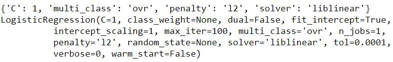
Fig — Best attributes of the Logistic Regression
We can observe that the best hyper parameters are as follows.
{'C': 1, 'multi_class': 'ovr', 'penalty': 'l2', 'solver': 'liblinear'}We can feed the best parameters to the Logistic Regression model and observe whether it’s accuracy has increased.
logreg_new = LogisticRegression(C=1, multi_class='ovr', penalty='l2', solver='liblinear')

initial_score = cross_val_score(logreg_new, X_new, y,
cv=strat_k_fold, scoring='accuracy').mean()
print("Final accuracy : {} ".format(initial_score))

Final accuracy : 0.7805877119643279
We could conclude that the hyper parameter tuning didn’t increase it’s accuracy. Maybe the hyper parameters we chose weren’t indicative. However you are welcome to try adding more parameter combinations.
The most important aspect is the procedure of doing hyper parameter tuning, not the result it self. In most cases hyper parameter tuning increases the accuracy.
We manage to achieve a classification accuracy of 78.05% which we can say is quite good.
Conclusion
We have reached the end of the article series. In this series we went through the entire machine learning workflow. We discussed the theory and the practical knowledge needed to complete a classification task.
We discussed about the machine learning workflow steps such as data exploration, data cleaning steps, feature engineering basics and advanced feature selections, model selection and hyper parameter tuning using Scikit Learn library.
It’s your turn now! Now you should be able to use this knowledge to try out other data sets.
Source: Medium
The Tech Platform


Comments