Linear Regression — Detailed View
- The Tech Platform

- Feb 17, 2021
- 5 min read
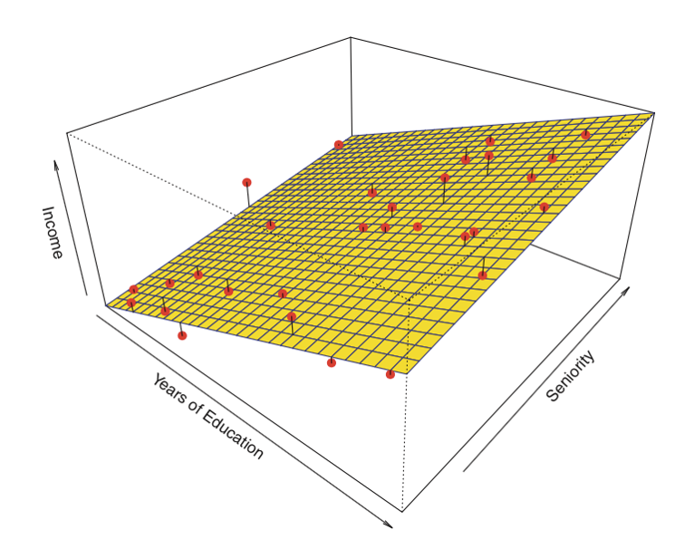
Linear regression is used for finding linear relationship between target and one or more predictors. There are two types of linear regression- Simple and Multiple.
Simple Linear Regression
Simple linear regression is useful for finding relationship between two continuous variables. One is predictor or independent variable and other is response or dependent variable. It looks for statistical relationship but not deterministic relationship. Relationship between two variables is said to be deterministic if one variable can be accurately expressed by the other. For example, using temperature in degree Celsius it is possible to accurately predict Fahrenheit. Statistical relationship is not accurate in determining relationship between two variables. For example, relationship between height and weight.
The core idea is to obtain a line that best fits the data. The best fit line is the one for which total prediction error (all data points) are as small as possible. Error is the distance between the point to the regression line.
Real-time example
We have a dataset which contains information about relationship between ‘number of hours studied’ and ‘marks obtained’. Many students have been observed and their hours of study and grade are recorded. This will be our training data. Goal is to design a model that can predict marks if given the number of hours studied. Using the training data, a regression line is obtained which will give minimum error. This linear equation is then used for any new data. That is, if we give number of hours studied by a student as an input, our model should predict their mark with minimum error.
Y(pred) = b0 + b1*x
The values b0 and b1 must be chosen so that they minimize the error. If sum of squared error is taken as a metric to evaluate the model, then goal to obtain a line that best reduces the error.
Figure 2: Error Calculation
If we don’t square the error, then positive and negative point will cancel out each other.
For model with one predictor,
Figure 3: Intercept Calculation
Figure 4: Co-efficient Formula
Exploring ‘b1’
If b1 > 0, then x(predictor) and y(target) have a positive relationship. That is increase in x will increase y.
If b1 < 0, then x(predictor) and y(target) have a negative relationship. That is increase in x will decrease y.
Exploring ‘b0’
If the model does not include x=0, then the prediction will become meaningless with only b0. For example, we have a dataset that relates height(x) and weight(y). Taking x=0(that is height as 0), will make equation have only b0 value which is completely meaningless as in real-time height and weight can never be zero. This resulted due to considering the model values beyond its scope.
If the model includes value 0, then ‘b0’ will be the average of all predicted values when x=0. But, setting zero for all the predictor variables is often impossible.
The value of b0 guarantee that residual have mean zero. If there is no ‘b0’ term, then regression will be forced to pass over the origin. Both the regression co-efficient and prediction will be biased.
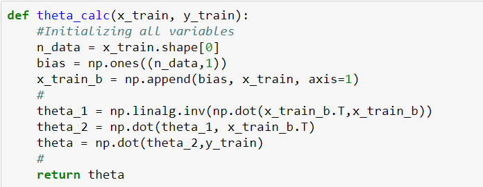
Co-efficient from Normal equations
Apart from above equation co-efficient of the model can also be calculated from normal equation.
Figure 5: Co-efficient calculation using Normal Equation
Theta contains co-efficient of all predictors including constant term ‘b0’. Normal equation performs computation by taking inverse of input matrix. Complexity of the computation will increase as the number of features increase. It gets very slow when number of features grow large.
Below is the python implementation of the equation.
Figure 6: Python implementation of Normal Equation
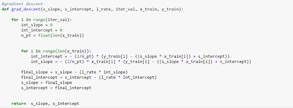
Optimizing using gradient descent
Complexity of the normal equation makes it difficult to use, this is where gradient descent method comes into picture. Partial derivative of the cost function with respect to the parameter can give optimal co-efficient value.
Python code for gradient descent
Figure 7: Python Implementation of gradient descent
Residual Analysis
Randomness and unpredictability are the two main components of a regression model.
Prediction = Deterministic + Statistic
Deterministic part is covered by the predictor variable in the model. Stochastic part reveals the fact that the expected and observed value is unpredictable. There will always be some information that are missed to cover. This information can be obtained from the residual information.
Let’s explain the concept of residue through an example. Consider, we have a dataset which predicts sales of juice when given a temperature of place. Value predicted from regression equation will always have some difference with the actual value. Sales will not match exactly with the true output value. This difference is called as residue.
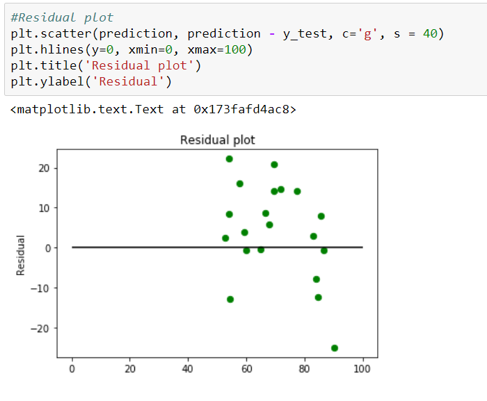
Residual plot helps in analyzing the model using the values of residues. It is plotted between predicted values and residue. Their values are standardized. The distance of the point from 0 specifies how bad the prediction was for that value. If the value is positive, then the prediction is low. If the value is negative, then the prediction is high. 0 value indicates prefect prediction. Detecting residual pattern can improve the model.
Non-random pattern of the residual plot indicates that the model is,
Missing a variable which has significant contribution to the model target
Missing to capture non-linearity (using polynomial term)
No interaction between terms in model
Characteristics of a residue
Residuals do not exhibit any pattern
Adjacent residuals should not be same as they indicate that there is some information missed by system.
Residual implementation and plot
Figure 8: Residual Plot
Metrics for model evaluation
R-Squared value
This value ranges from 0 to 1. Value ‘1’ indicates predictor perfectly accounts for all the variation in Y. Value ‘0’ indicates that predictor ‘x’ accounts for no variation in ‘y’.
1. Regression sum of squares (SSR)
This gives information about how far estimated regression line is from the horizontal ‘no relationship’ line (average of actual output).
Figure 9: Regression Error Formula
2. Sum of Squared error (SSE)
How much the target value varies around the regression line (predicted value).
Figure 10: Sum of Square Formula
3. Total sum of squares (SSTO)
This tells how much the data point move around the mean.
Figure 11: Total Error Formula
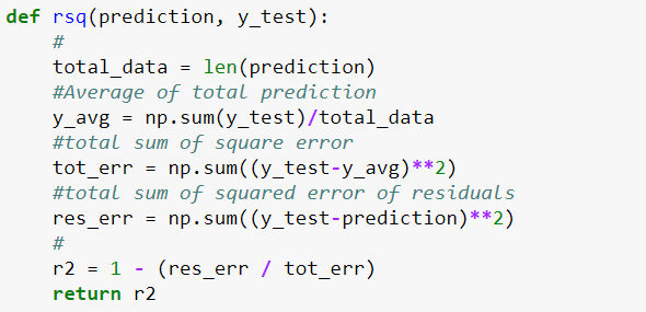
Python implementation
Figure 12: Python Implementation of R-Square
Is the range of R-Square always between 0 to 1?
Value of R2 may end up being negative if the regression line is made to pass through a point forcefully. This will lead to forcefully making regression line to pass through the origin (no intercept) giving an error higher than the error produced by the horizontal line. This will happen if the data is far away from the origin.
Correlation co-efficient (r)
This is related to value of ‘r-squared’ which can be observed from the notation itself. It ranges from -1 to 1.
r = (+/-) sqrt(r²)
If the value of b1 is negative, then ‘r’ is negative whereas if the value of ‘b1’ is positive then, ‘r’ is positive. It is unitless.
Null-Hypothesis and P-value
Null hypothesis is the initial claim that researcher specify using previous research or knowledge.
Low P-value: Rejects null hypothesis indicating that the predictor value is related to the response
High P-value: Changes in predictor are not associated with change in target
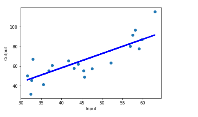
Obtained Regression line
Figure 13: Final Regression line over test data
Full code: https://github.com/SSaishruthi/Linear_Regression_Detailed_Implementation
This is an educational post made by complilation of materials (like Prof.Andrew Ng course, Siraj Raval’s videos, etc. ) that helped me in my journey. Other references are stated near the content.
Source: datascience
The Tech Platform











Comments