Insertion Sort Algorithm

Insertion sort is a simple sorting algorithm that builds the final sorted array one element at a time. It is an in-place and stable sorting algorithm, meaning it does not require additional memory and preserves the relative order of equal elements in the sorted array.

The basic idea behind insertion sort is to divide the input array into a sorted and an unsorted part. Initially, the sorted part contains only the first element, and the unsorted part contains the rest of the elements. The algorithm then iterates through the unsorted part, taking one element at a time and inserting it into its correct position in the sorted part.

Pseudocode

INSERTION-SORT(A)
   for i = 1 to n
   	key ← A [i]
    	j ← i – 1
  	 while j > = 0 and A[j] > key
   		A[j+1] ← A[j]
   		j ← j – 1
   	End while 
   	A[j+1] ← key
  End for 

How does it work?

Here's a step-by-step explanation of how the Insertion Sort algorithm works:

1. Start with the first element, which is the sorted part of the array.

2. Take the next element from the unsorted part.

3. Compare the current element with the elements in the sorted part from right to left.

4. Move the larger elements to the right until the correct position for the current element is found.

5. Insert the current element into its correct position in the sorted part.

6. Repeat steps 2-5 until all elements are in their appropriate positions.

This process continues until all elements are sorted, and the array is arranged in ascending order. The algorithm works in-place, meaning it does not require additional memory to sort the array, and it is also stable, preserving the relative order of equal elements.

Implementation

Let's create the step-by-step working of the Insertion Sort algorithm with the given example:

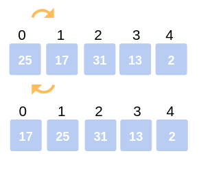
Consider the following array: 25, 17, 31, 13, 2

STEP 1: First Iteration: Compare 25 with 17. The comparison shows 17 < 25. Hence, swap 17 and 25. Array becomes: 17, 25, 31, 13, 2.

First Iteration

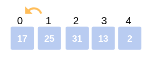
STEP 2: Second Iteration: Move on to the second element (25). It was already swapped for the correct position, so move to the next element.

STEP 3: Hold the third element (31) and compare it with the ones preceding it. Since 31 > 25, no swapping takes place. Also, 31 > 17, no swapping takes place, and 31 remains at its position. Array remains: 17, 25, 31, 13, 2

Second Iteration

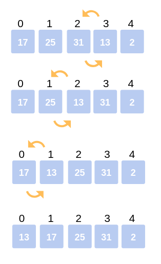
STEP 4: Third Iteration: Start the next iteration with the fourth element (13) and compare it with its preceding elements. Since 13 < 31, swap the two. Array becomes: 17, 25, 13, 31, 2.

Now, there are still elements that haven't been compared with 13. The comparison takes place between 25 and 13. Since 13 < 25, swap the two. Array becomes: 17, 13, 25, 31, 2.

The last comparison for this iteration is between 17 and 13. Since 13 < 17, swap the two. Array becomes: 13, 17, 25, 31, 2.

Third Iteration

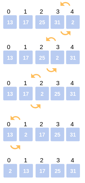
STEP 5: Fourth Iteration: The last iteration calls for the comparison of the last element (2) with all the preceding elements and make the appropriate swapping between elements. Since 2 < 31, swap 2 and 31. Array becomes: 13, 17, 25, 2, 31.

Compare 2 with 25, 17, 13. Since 2 < 25, swap 25 and 2. Array becomes: 13, 17, 2, 25, 31.

Compare 2 with 17 and 13. Since 2 < 17, swap 2 and 17. Array becomes: 13, 2, 17, 25, 31.

The last comparison for this iteration is to compare 2 with 13. Since 2 < 13, swap 2 and 13. Array becomes: 2, 13, 17, 25, 31.

This is the final array after all the corresponding iterations and swapping of elements. It is now sorted in ascending order using the Insertion Sort algorithm.

Fourth Iteration

Characteristics of Insertion Sort

1. It is efficient for smaller data sets: Insertion Sort performs relatively well on small arrays or partially sorted data compared to other sorting algorithms like Merge Sort or Quick Sort.

2. Adaptive: Insertion Sort is adaptive, which means it becomes more efficient if the input array is partially sorted. It reduces the number of steps required to sort the array in such cases.

3. Better than Selection Sort and Bubble Sort: In general, Insertion Sort outperforms algorithms like Selection Sort and Bubble Sort in terms of efficiency.

4. Space complexity: The space complexity of Insertion Sort is O(1), which means it requires only a constant amount of additional memory to perform the sorting in-place.

5. Stable sorting: Insertion Sort is a stable sorting technique, meaning it preserves the relative order of elements with equal values. If two elements have the same value, their original order is maintained in the sorted array.

Complexity Analysis of Insertion Sort

Worst-case time complexity (Big-O): O(n^2) - This occurs when the input array is in reverse order, and the maximum number of comparisons and swaps are required to sort the array.

Best-case time complexity (Big-Omega): O(n) - This occurs when the input array is already sorted. In this case, the inner loop performs fewer iterations since no swaps are needed, resulting in a linear time complexity.

Average time complexity (Big-Theta): O(n^2) - On average, Insertion Sort requires n^2 operations to sort an array of n elements, making it less efficient than some other sorting algorithms like Merge Sort or Quick Sort.

Space complexity: O(1) - As mentioned earlier, Insertion Sort only requires a constant amount of additional memory, making it an in-place sorting algorithm.

It's important to note that while Insertion Sort has some advantages, it is not the most efficient sorting algorithm for large datasets due to its quadratic time complexity. For larger arrays, more advanced algorithms like Merge Sort or Quick Sort are generally preferred.